
L&R Frequency Estimation (II)
I finished the last note with the expression presented by Louise and Reggiannini (L&R) in 1995 for the estimation of the frequency of a complex sinusoid:
\[\hat{f_n} = {\frac{1}{\pi(M+1)}} \operatorname{arg} \left\{ \sum_{i=1}^{M} R(k) \right\}\]with
\[R(k) \triangleq {\frac{1}{N-k}}\sum_{i=1}^{N-k} s_{i+k} s^{*}_{i}\]\(s_{i} = e^{j(2\pi f_n i + \theta_0)}\) are the samples of our complex sinusoid signal, and \(f_n\) and \(\hat{f_n}\) are the true and estimated frequencies of our signal, respectively. We have \(N\) consecutive samples available and there is a configuration parameter \(M\) with \(M \leq N-1\). The accuracy of the method, as well as it computational complexity, depends on the choice of \(M\) and, as expected, there is a trade-of between both. I have been concerned with this trade-off lately. I’ll try to convey in this note what I have learned so far.
As explained before, \(R(k)\) compute the signal auto-correlation at a gap of \(k\) samples. Considering that our complex sinusoid is affected by additive noise \(n\), our \(s_{i+k} s^{*}_{i}\) auto-correlation products can be expressed as:
\[s_{i+k} s^{*}_{i} = (e^{j(2\pi f_n (i+k) + \theta_0)} + n_{i+k})(e^{-j(2\pi f_n i + \theta_0)} + n^{*}_{i})\] \[= e^{j 2\pi f_n k} + n_{i+k}e^{-j(2\pi f_n k + \theta_0)} + n^{*}_{i}e^{j(2\pi f_n (i+k) + \theta_0)} + n_{i+k}n^{*}_{i}\]We can replace the first-order noise components by a rotated version of them, with their same statistical properties:
\[= e^{j 2\pi f_n k} + n_{i+k}^{\prime*} + n_{i}^{\prime*} + n_{i+k}n^{*}_{i} \tag{1}\label{eq:1}\]Remember that our frequency estimation consist of adding together a bunch of these terms and calculating the angle of the result. It’s intuitive then to say that for small gap values \(k\), our \(e^{j 2\pi f_n k}\) is going to be near the real axis and the angle of our expression (1) is dominated by the noise components. Larger values of \(k\) make our \(e^{j 2\pi f_n k}\) stand out and should produce better estimates of \(f_n\). The challenge here is that in the \(R\) summation there are only a few auto-correlation terms at large \(k\) (e.g.: with \(N=10\), there is only one auto-correlation term at gap \(k=9\), which is \(s_{10} s^{*}_{1}\)). There are, however, many terms at lower \(k\) (e.g.: there are nine terms at \(k=1\): \(s_{2} s^{*}_{1}, s_{3} s^{*}_{2}, ... s_{10} s^{*}_{9}\)). So, there is a tension: terms at short gaps are more noisy, but we are adding more, which lowers the overall noisiness. Terms at bigger gaps are less noisy, but we have fewer to add, so it’s not so clear where is the sweet spot. Let’s explore this.
The term \(M\) is the upper bound for the gaps we are going to use. Based on the previous, I had the idea (most likely not the first one to tread this path) that there should also be a lower bound:
\[\hat{f_n} = {\frac{1}{\pi(M+1)}} \operatorname{arg} \left\{ \sum_{i=m_{1}}^{m_{2}} R(k) \right\}\]It would be interesting to see what’s the expected accuracy in the frequency estimate with different \(m1, m2\) values. I don’t have the math belt level required to come up with the analytical expression, but fortunately these days we have computers to help us run a bunch of simulations: adding white noise to a sinusoid to make its SNR equal to 3 dB and with \(N\)=90 samples, the following chart represents the estimated RMS error with 100k trials for different values of \(m1\) and \(m2\):
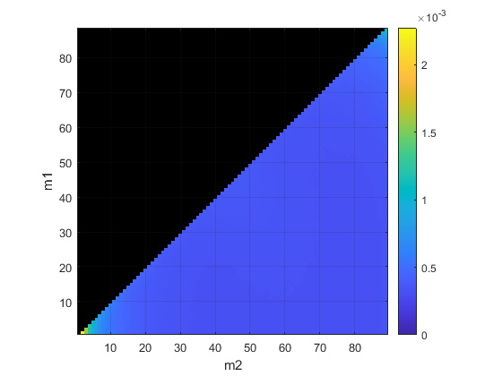
(\(m1\) is in the range \([1, N-2]\) and \(m2\) in \([m1+1, N-1]\))
A contour plot is more helpful to understand how the RMS error changes:
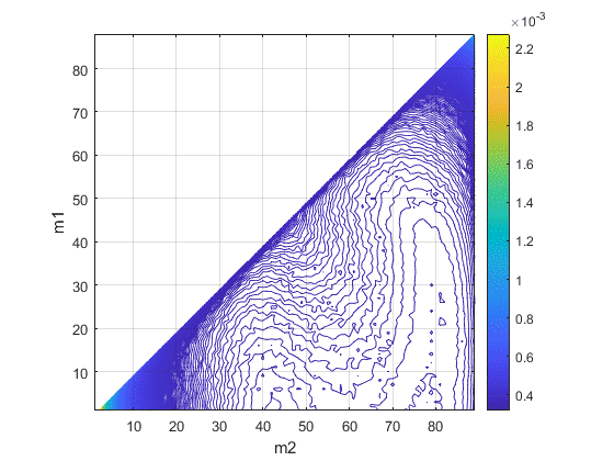
It’s remarkable to see that lowest RMS error (about 3.2e-4 in normalized frequency units) is achieved at (\(m1\),\(m2\))=(1,41) and that there is another local minima at (1,79):
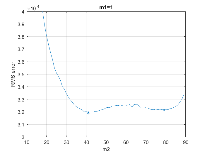
The practical difference between these points is very small and their location should be dependent with the actual SNR of our signal. The number of computations at \(m2\)=41 is significantly smaller than at \(m2\)=79, so, under these results, it seems sensible to abandon the idea of having two bounds \(m1,m2\). We should go back to the original L&R formulation with a single parameter \(M\), making it a bit below \(N/2\), at least for this particular SNR level.
To complete the analysis, let’s take a look at some simulations. Next one is run with 100k trials, no frequency offset is applied to the signal (so the signal is a carrier with a frequency of 0 Hz, or just a constant value), \(N\)=90 and \(M\)=41, at different SNR points:
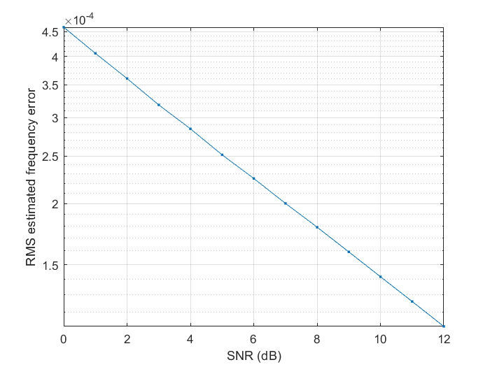
The straight line that we see in this log plot is the signature of the quality of this estimate. The major constraint that we are going to find comes from the maximum tolerated frequency error. In this case with \(M\)=41 we are limited by a frequency error of 0.5/41 = 0.012195 normalized frequency units. We can see that on the following chart:
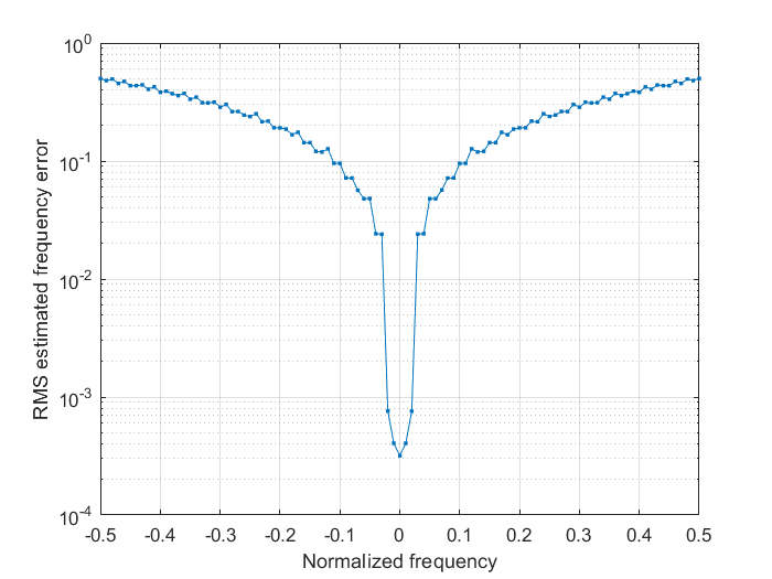
The SNR is fixed to 3 dB and, again, \(N\)=90 and \(M\)=41. Zooming in we get a better insight:
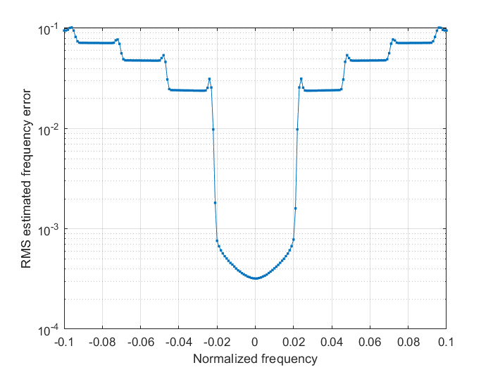
In practice it looks that we have a bit more margin and the method is working inside the [-0.02,0.02] range, but don’t try your luck and, for this particular choice of \(N\) and \(M\), try to stay within the recommended [-0.01295, 0.012195] limits.
Bonus material
Trying different ideas, I was able to calculate the exact formula for the RMS error derived from individual \(R(k)\). As I will explain later, this turned out not very useful. Anyway, it might be in a future work and I have decided to keep it.
We start by realizing that we need to consider the additive noise component and noise and signal power, so we reboot the analysis defining our complex sinusoid as:
\[s_{i} = \sigma_{s} e^{j(2 \pi f_{n} i + \theta_{0})}, 1 \leq i \leq N\]with power \(\sigma^{2}_{s}\). We keep the definition of our auto-correlation function \(R(k)\):
\[R(k) \triangleq {\frac{1}{N-k}}\sum_{i=1}^{N-k} r_{i+k} r^{*}_{i} \tag{2}\label{eq:2}\]Here \(r=s+n\), being \(n\) the additive Gaussian noise component in our received signal.
We have already seen that, if our noise is negligible, \(R(k)\) is approximated by:
\[R(k) \approx \sigma^{2}_{s} e^{j2 \pi f_{n} k}\]and then we could use it to produce an estimate of our \(f_{n}\):
\[\hat{f_{n}} = {\frac{\operatorname{arg}(R(k))}{2 \pi k}} \tag{3}\label{eq:3}\]What follows is the excruciating derivation of the analytical expression of the RMS error of this estimate at any given SNR level.
OK, so they point is that we can’t keeping ignore the noise component. Expanding \(r\) in eq. (2) we get:
\[R(k) = {\frac{1}{N-k}}\sum_{i=1}^{N-k}(\sigma_{s} e^{j(2 \pi f_{n} (i+k) + \theta_{0})} + n_{i+k})(\sigma_{s} e^{-j(2 \pi f_{n} i + \theta_{0})} + n_{i}^{*})\]which we can understand as the sum of three components:
\[R(k) = T_{0}(k) + T_{1}(k) + T_{2}(k)\]\(T_{0}\) is our “signal” component, the same one we obtained in the no-noise scenario:
\[T_{0}(k) = \sigma^{2}_{s} e^{j2 \pi f_{n} k}\]\(T_{1}\) is our first-order noise component:
\[T_{1}(k) = {\frac{\sigma_{s}}{N-k}} \left( \sum_{i=1}^{N-k} e^{j (2 \pi f_{n} (i+k) + \theta_{0})} n_{i}^{*} + \sum_{i=1}^{N-k} e^{-j (2 \pi f_{n} i + \theta_{0})} n_{i+k} \right)\]and \(T_{2}\) is our second-order noise component:
\[T_{2}(k) = {\frac{1}{N-k}}\sum_{i=1}^{N-k} n_{i+k}n_{i}^{*}\]Taking this into (3), we can expand our frequency estimate as
\[\hat{f}_{n} = {\frac{\operatorname{arg}(\sigma^{2}_{s} e^{j2 \pi f_{n} k} + T_{1}(k) + T_{2}(k))}{2 \pi k}}\] \[= f_{n} + {\frac{\operatorname{arg}(\sigma^{2}_{s} + e^{-j2 \pi f_{n} k}(T_{1}(k) + T_{2}(k)))}{2 \pi k}} \tag{4}\label{eq:4}\]This makes evident that the noise in our estimate comes from the \(T_{1}\) and \(T_{2}\) components.
We are going to tackle \(T_{1}\) first. We can’t make more progress without realizing that that there is overlap in the \(T_{1}\) summations. To make it explicit we need to split the intervals in \([1,k]\), \([k+1,N-k]\) and \([1,N-2k]\), \([N-2k+1,N-k]\)
\[\begin{align*} T_{1}(k) = {\frac{\sigma_{s}}{N-k}} \left( \sum_{i=1}^{k} e^{j (2 \pi f_{n} (i+k) + \theta_{0})} n_{i}^{*} + \sum_{i=k+1}^{N-k} e^{j (2 \pi f_{n} (i+k) + \theta_{0})} n_{i}^{*} + \\ \sum_{i=1}^{N-2k} e^{-j (2 \pi f_{n} i + \theta_{0})} n_{i+k} + \sum_{i=N-2k+1}^{N-k} e^{-j (2 \pi f_{n} i + \theta_{0})} n_{i+k} \right) \end{align*}\]Modifying the summation indexes so all the summations are expressed in terms of \(n_{i}\) we get:
\[\begin{align*} T_{1}(k) = {\frac{\sigma_{s}}{N-k}} \left( \sum_{i=1}^{k} e^{j (2 \pi f_{n} (i+k) + \theta_{0})} n_{i}^{*} + \sum_{i=k+1}^{N-k} e^{j (2 \pi f_{n} (i+k) + \theta_{0})} n_{i}^{*} + \\ \sum_{i=k+1}^{N-k} e^{-j (2 \pi f_{n} (i-k) + \theta_{0})} n_{i} + \sum_{i=N-k+1}^{N} e^{-j (2 \pi f_{n} (i-k) + \theta_{0})} n_{i} \right) \end{align*}\]Which shows that we can factor out the term \(e^{j 2 \pi f_{n} k}\)
\[\begin{align*} T_{1}(k) = {\frac{\sigma_{s} e^{j 2 \pi f_{n} k} }{N-k}} \left(\sum_{i=1}^{k} e^{j (2 \pi f_{n} i + \theta_{0})} n_{i}^{*} + \sum_{i=k+1}^{N-k} e^{j (2 \pi f_{n} i + \theta_{0})} n_{i}^{*} + \\ \sum_{i=k+1}^{N-k} e^{-j (2 \pi f_{n} i + \theta_{0})} n_{i} + \sum_{i=N-k+1}^{N} e^{-j (2 \pi f_{n} i + \theta_{0})} n_{i} \right) \tag{5}\label{eq:5} \end{align*}\]The second and third summation can be combined. We are going to use the following:
\[e^{j (2 \pi f_{n} i + \theta_{0})} n_{i}^{*} + e^{-j (2 \pi f_{n} i + \theta_{0})} n_{i} = (e^{-j (2 \pi f_{n} i + \theta_{0})} n_{i})^{*} + e^{-j (2 \pi f_{n} i + \theta_{0})} n_{i}\]The noise terms are rotated and a rotation is not going to alter their statistical properties. We can define
\[n_{i}^{\prime} \triangleq e^{-j (2 \pi f_{n} i + \theta_{0})} n_{i}\]so
\[n_{i}^{\prime*} + n_{i}^{\prime} = 2 \operatorname{Re}(n_{i}^{\prime})\]and using this, (5) becomes
\[T_{1}(k) = {\frac{\sigma_{s} e^{j 2 \pi f_{n} k} }{N-k}} \left(\sum_{i=1}^{k} e^{j (2 \pi f_{n} i + \theta_{0})} n_{i}^{*} + 2\sum_{i=k+1}^{N-k} \operatorname{Re}(n_{i}^{\prime}) + \sum_{i=N-k+1}^{N} e^{-j (2 \pi f_{n} i + \theta_{0})} n_{i} \right) \tag{6}\label{eq:6}\]Let’s take a moment now to recap that our noise is Gaussian, with zero mean and power \(\sigma_{n}^{2}\). This is expressed more formally as
\[Noise \sim \mathcal{CN}(0,\sigma_{n}^{2})\]our noise is also complex-valued, so if we were to consider only its real component, we will see that
\[\operatorname{Re}(Noise) \sim \mathcal{N}(0,{\frac{\sigma_{n}^{2}}{2}})\]Back to (6), when \(N \geq 2k\), the intervals \([1,k]\) and \([N-k+1,N]\) don’t overlap, then, with the purpose of estimating the power components we can say that
\[T_{1}(k) \sim {\frac{\sigma_{s} e^{j 2 \pi f_{n} k} }{N-k}} \left(\mathcal{CN}(0,k\sigma_{n}^{2}) + 2\mathcal{N}(0,{\frac{(N-2k)\sigma_{n}^{2}}{2}}) + \mathcal{CN}(0,k\sigma_{n}^{2}) \right)\]or
\[T_{1}(k) e^{-j 2 \pi f_{n} k} \sim {\frac{\sigma_{s} }{N-k}} \left( \mathcal{CN}(0,2k\sigma_{n}^{2}) + 2\mathcal{N}(0,{\frac{(N-2k)\sigma_{n}^{2}}{2}}) \right)\]We are almost there. We can go back and apply the same approach to our \(T_{2}\) to get
\[T_{2}(k) \sim {\frac{1}{N-k}} \left( \mathcal{CN}(0,(N-k)\sigma_{n}^{4}) \right)\]or
\[T_{2}(k) e^{-j 2 \pi f_{n} k} \sim {\frac{1}{N-k}} \left( \mathcal{CN}(0,(N-k)\sigma_{n}^{4})\right)\]So we are finally in a position to bring all of these to our frequency error expression from (4)
\[\begin{align*} \hat{f}_{n} - f_{n} \sim {\frac{1}{2\pi k}} \operatorname{arg} \left( \sigma^{2}_{s} + {\frac{\sigma_{s} }{N-k}} \left( \mathcal{CN}(0,2k\sigma_{n}^{2}) + 2\mathcal{N}(0,{\frac{(N-2k)\sigma_{n}^{2}}{2}}) \right) + \\ {\frac{1}{N-k}} \left( \mathcal{CN}(0,(N-k)\sigma_{n}^{4})\right) \right) \end{align*}\] \[\begin{align*} \sim {\frac{1}{2\pi k}} \operatorname{arg} \left( \sigma^{2}_{s} + {\frac{1}{N-k}} \left( \sigma_{s} \left( \mathcal{CN}(0,2k\sigma_{n}^{2}) + 2\mathcal{N}(0,{\frac{(N-2k)\sigma_{n}^{2}}{2}}) \right) + \\ \mathcal{CN}(0,(N-k)\sigma_{n}^{4}) \right) \right) \end{align*}\]which can be simplified assuming that the signal power is significantly higher than the noise power and then the error is going to be determined mainly by the imaginary components in our noise, so
\[\hat{f}_{n} - f_{n} \sim {\frac{1}{2\pi k}} \operatorname{arg} \left( \sigma^{2}_{s} + {\frac{j}{N-k}} \left( \sigma_{s} \mathcal{N}(0,k\sigma_{n}^{2}) + \mathcal{N}(0,{\frac{(N-k)\sigma_{n}^{4}}{2}}) \right) \right)\]this is further simplified assuming that the angle is small so \(\operatorname{arg}(x+jy) \approx {\frac{y}{x}}\), getting
\[\hat{f}_{n} - f_{n} \sim {\frac{1}{2\pi k (N-k)\sigma_{s}^{2}}} \left( \sigma_{s} \mathcal{N}(0,k\sigma_{n}^{2}) + \mathcal{N}(0,{\frac{(N-k)\sigma_{n}^{4}}{2}}) \right)\]We are finally ready to compute the variance in our frequency estimate error, remembering that \(\operatorname{var}(a \mathcal{N}(0,\sigma^{2}))\) with \(a \in \mathbb{R}\) is \(a^{2}\sigma^{2}\)
\[\operatorname{var}(\hat{f}_{n} - f_{n}) \approx \left( {\frac{1}{2\pi k (N-k)\sigma_{s}^{2}}} \right)^{2} \left( \sigma_{s}^{2}k\sigma_{n}^{2} + {\frac{(N-k)\sigma_{n}^{4}}{2}} \right)\]Let’s call \(\rho\) to our signal-to-noise ratio, \(\rho = {\frac{\sigma_{s}^{2}}{\sigma_{n}^{2}}}\)
\[\operatorname{var}(\hat{f}_{n} - f_{n}) \approx {\frac{1}{4\pi^{2} k^{2} (N-k)\rho}} \left( {\frac{k}{N-k}} + {\frac{1}{2\rho}} \right) \tag{7}\label{eq:7}\]which we should remember is only valid for \(N \geq 2k\).
We consider now the case \(N < 2k\). Here we need to do some work on our \(T_{1}\) since the two terms:
\[S_{1} = \sum_{i=1}^{k} e^{j (2 \pi f_{n} i + \theta_{0})} n_{i}^{*}\]and
\[S_{2} = \sum_{i=N-k+1}^{N} e^{-j (2 \pi f_{n} i + \theta_{0})} n_{i}\]overlap. This overlap is going to produce a similar effect to what we have already seen: part of the noise along the imaginary component is going to cancel out, which is good news. This is revealed splitting the summations in the \([1, N-k]\), \([N-k+1, k]\) and \([N-k+1, k]\), \([k, N]\) respectively:
\[S_{1} = \sum_{i=1}^{N-k} e^{j (2 \pi f_{n} i + \theta_{0})} n_{i}^{*} + \sum_{i=N-k+1}^{k} e^{j (2 \pi f_{n} i + \theta_{0})} n_{i}^{*}\]and
\[S_{2} = \sum_{i=N-k+1}^{k} e^{-j (2 \pi f_{n} i + \theta_{0})} n_{i} + \sum_{i=k}^{N} e^{-j (2 \pi f_{n} i + \theta_{0})} n_{i}\]The \([N-k+1, k]\) is the overlapping interval, which we know is properly formed since \(N < 2k\) and so \(N-k+1 < k+1\).
Adding everything together:
\[S_{1} + S_{2} = \sum_{i=1}^{N-k} e^{j (2 \pi f_{n} i + \theta_{0})} n_{i}^{*} + \sum_{i=N-k+1}^{k} \left( (e^{-j (2 \pi f_{n} i + \theta_{0})} n_{i})^{*} + e^{-j (2 \pi f_{n} i + \theta_{0})} n_{i} \right) + \sum_{i=k+1}^{N} e^{-j (2 \pi f_{n} i + \theta_{0})} n_{i}\]and using the same approach we followed earlier:
\[S_{1} + S_{2} = \sum_{i=1}^{N-k} e^{j (2 \pi f_{n} i + \theta_{0})} n_{i}^{*} + 2\sum_{i=N-k+1}^{k} \operatorname{Re}(n_{i}^{\prime}) + \sum_{i=k+1}^{N} e^{-j (2 \pi f_{n} i + \theta_{0})} n_{i}\]As before, we are only interested in the imaginary component and this behaves as
\[\mathcal{N}(0,(N-k)\sigma_{n}^{2})\]So we end up with
\[\operatorname{Im}(T_{1}(k) e^{-j 2 \pi f_{n} k}) \sim {\frac{\sigma_{s} }{N-k}} \mathcal{N}(0,(N-k)\sigma_{n}^{2})\]and so
\[\operatorname{var}(\hat{f}_{n} - f_{n}) \approx \left( {\frac{1}{2\pi k (N-k)\sigma_{s}^{2}}} \right)^{2} \left( \sigma_{s}^{2}(N-k)\sigma_{n}^{2} + {\frac{(N-k)\sigma_{n}^{4}}{2}} \right)\]and we finally get
\[\approx {\frac{1}{4\pi^{2} k^{2} (N-k)\rho}} \left( 1 + {\frac{1}{2\rho}} \right)\]valid when \(N < 2k\).
Taking this together with (7) we reach what we wanted, an analytical (approximated) expression for the variance in our error when we use (3) to estimate the frequency of our complex sinusoid:
\[\operatorname{var}(\hat{f}_{n} - f_{n}) \approx \left\{ \begin{array}{ll} {\frac{1}{4\pi^{2} k^{2} (N-k)\rho}} \left( {\frac{k}{N-k}} + {\frac{1}{2\rho}} \right) & k \leq N/2 \\ {\frac{1}{4\pi^{2} k^{2} (N-k)\rho}} \left( 1 + {\frac{1}{2\rho}} \right) & k > N/2 \\ \end{array} \right. \tag{8}\label{eq:8}\]being \(\rho\) our complex sinusoid SNR (which is then probably more appropriate to refer to it as CNR or carrier-to-noise ratio).
We can compare this with results from simulations. The following chart was produced with \(N=90\), SNR 3 dB and 60k trials:
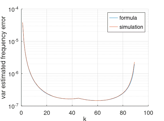
Seems like it’s accurate. This is also a confirmation of the intuition that was presented at the beginning of this note: low and high \(k\) values produce low quality estimates, intermediate values give better results, at least when the \(R(k)\) are considered individually.
Indeed an interesting result and my initial idea was to use it as an alternative way to compute the variance in the estimation error for the L&R method. Since the L&R method is based on the addition of a number of \(R(k)\), it should be easy to derive it from (8). To say that is a mistake since the \(R(k)\) are correlated to each other. If we calculate the covariance matrix of the \(R(k)\) on the same 60k trial simulation, we get values outside the main diagonal:
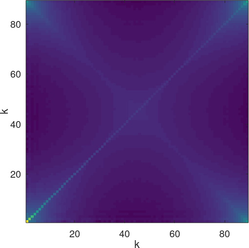
I think that it makes sense to say that neighboring \(k\) values are correlated to each other, and it’s probably going to be complicated to quantify that correlation, so don’t I think this line of thought is going to get us very far and I won’t pursue it at this point.
Kudos to L&R for their insight and hard work. Things are much easier now with affordable computers to do the heavy lifting for us, they didn’t have this luxury 30 years ago. I finish this note with my appreciation.
Leave a Comment