Embracing Doing Nothing

“Less is more.” The tension between more sophisticated processing versus lower power consumption and cheaper components tilts the balance towards simpler and more effective solutions. We like to call them “elegant.” The pinnacle of elegance is then achieved when we realize that the problem we are trying to solve doesn’t need to be solved. This realization is usually the destination of a long journey, even longer when we consider the amount of convincing that will be involved. Nobody questions when more complexity is added to the machine, but do we have enough confidence to propose the removal of a critical component?

I’ve been in this situation not long ago and I think it is worth it to clean up my notes and put them in writing. This story is in the symbol timing tracking topic, which it happens that I have covered a few times, for instance reviewing some of the classical algorithms such as M&M or D’Andrea.

Symbol timing tracking is a critical piece in our overarching task of recovering the digital content of a radio signal. Using the following “eye diagram” as reference:

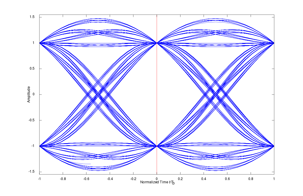Image credit: Wikipedia

we see that the maximum gap in the “eye” corresponds to the 0 point in the x-axis, representing the normalized symbol timing (aka symbol timing phase). There lies our best chance. At any other sampling point the gap in the eye will be smaller, indicating a penalty in the signal SNR. Notice how the eye is completely closed at ±0.5. With such a bad timing error, we have a 50% chance of recovering our data. This is no better than a coin toss and we don’t want to be there.

The tracking of the symbol timing is important because transmitter and receiver run with different, unsynchronized clocks, so, even if we manage to achieve a pretty good initial symbol timing estimation, the different pace of the clocks will make it drift, forward or backwards, and we will see how our signal quality drops until the point the eye closes too much and we lose it.

Let’s consider symbol timing tracking in the context of another topic that I’ve also covered several times: AIS. AIS is a maritime safety system that ships use to broadcast its location (coming from a GPS receiver) among other important information (speed, bearing, etc.). AIS was developed in the 1990s and it uses practical technology from this date, which predates the era of SDR and more sophisticated communication systems. The signal specs for our purposes in this note, can be summarized as:

• GMSK modulation.
• 9600 baud.
• Typical message length is 168 bits, including training sequence, markers and other overheads, about 200 symbols (“symbol” and “bit” are used interchangeably here since GMSK encodes one bit per symbol.)
• Frequency band: around 162 MHz.

Tasked with designing a symbol tracking module for AIS, we should invest in studying the about 150 pages of the standard (recommendation ITU-R M.1371-5 (02/2014)), to find this relevant requirement on the AIS transmitter:

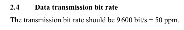
This ppm means “parts per million,” so an AIS transponder is expected to transmit at a symbol rate within the [9599.99995, 9600.00005] baud range. This means that, worst-case, after 1/50e-6 = 20k seconds we are going to receive one bit less (or more) of what would be expected at the exact symbol rate of 9600 baud. In other words, after 20k seconds our symbol timing error is going to have accumulated to ±1 normalized units. Since we have already seen that an error of ±0.5 is critical, we should design our system to stay within a symbol timing error of, at most, [-0.25, 0.25] units. For a transmitter with a clock error rate of 50 ppm, starting with a perfect knowledge of the symbol timing (error = 0), the error will increase to 0.25 after 20k*0.25 = 5k seconds or about one hour and 23 minutes.

What does this mean in the context of an AIS message? You have probably noticed that, in practical matters, very little. Since our AIS message only last for about 21 ms (200 symbols / 9600 symbols/s = 20.83 ms), with an error rate of 50 ppm, after 21 ms we should expect a symbol timing error of 21e-3*50e-6 = 1.05e-6 normalized units, which in practice is nothing, much below our resolution.

However, this is only one half of the equation, the transmitting side. The other half comes from the receiving side. What’s the expected timing error rate on a typical SDR hardware? It depends. Amateur hardware is already coming out with decent specs, see for instance, the RTL-SDR V3 with a temperature-controlled crystal oscillator (TCXO) of ±1 ppm frequency stability, which is pretty good.

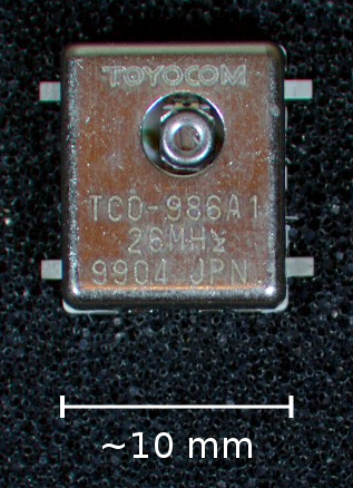“SMD Crystal Oscillator TCXO” by Appaloosa is licensed under CC BY 3.0.

In the context of frequency stability, ±1 ppm means that an oscillator labeled as 1 MHz should be expected to resonate at a frequency in the range of [999999, 1000001] Hz. Here is the starting point to translate this figure to a symbol timing error rate. The next step comes from understanding that in common SDR designs this oscillator is going to drive all the different clocks required by different hardware modules, including the important analog-to-digital converter (ADC). The ADC is programmed to run at some specific sampling rate and this sampling rate is derived from the oscillator using some phase-locked loop (PLL) or equivalent circuitry. The main idea is that the oscillator frequency is going to be multiplied by some rational number into our intended sampling rate.

It’s typical for a digital receiver to tune the sampling rate to a multiple of the sampling rate. This is called “oversampling” and a value of 4 samples per symbol is common. In our AIS example, the ADC will then be set to run at a sampling rate of 4*9600 = 38400 samples per second. With an uncertainty of ±1 ppm, it means that the actual sampling rate is going to be 38400*(1±1/1e6) = [38399.9616, 38400.0384] samples/s. Then, at the end of our AIS message, or in other words, after 20.83 ms, we should expect to have received 20.83e-3*[38399.9616, 38400.0384] = [799.9992, 800.0008], instead of the 20.83e-3*38400 = 800 samples that we would get with a perfect clock. The symbol timing error is then ±0.0008, still very small.

If you prefer a clean expression for this final figure, the development can be:

Uncentainty is additive and we can then say that the expected timing drift is the sum of transmitter and receiver, or 1.05e-6 + 0.0008 = 0.00080105. Still a very small number, which means that, having an accurate initial symbol timing estimation, we can get rid of the symbol timing tracking altogether. This is still true, even if we go back to the earlier versions of the RTL SDR dongles with abysmal frequency uncertainties of ±100 ppm or even worse.

But then, why do we see many AIS receivers implementing symbol timing tracking modules? What happens is that the designer might have decided not to invest in a good initial timing estimation or maybe to eliminate it altogether. The idea is that the symbol timing tracking of choice, applied to the very beginning of the AIS message should have enough time to synchronize by the time we get to the end of the training sequence. Still not being at this point so accurate, it can continue to improve along as the message goes, maybe taking advantage of a data-aided approach.

I will spend the next note presenting an alternative to these designers: a symbol timing estimator for AIS that offers enough accuracy, even under low SNR, so they can confidently dispense with the symbol timing tracking module and avoid solving a problem that doesn’t need to be solved.