
D’Andrea (1990) Clock Recovery
We are making slow progress here, finally reaching developments from the 90s. This post is concerned with the popular paper by D’Andrea, Mengali and Reggiannini from 1990, “A digital approach to clock recovery in generalized MSK.” Drs. Mengali and D’Andrea are also the authors of the expensive “Synchronization Techniques for Digital Receivers,” one of the few books in this specialized subject.
In this paper the authors develop a practical clock recovery method for MSK signals cleverly exploiting a pattern that shows in the complex base-band signal and is the basis for a number of derived methods that followed in the literature. Working in the complex domain is a change in this series, the other posts in this series recover the clock from the signal differential phase. This can be understood as an improvement since extracting the differential phase from the complex signal is inherently a noisy step, avoiding it can open the way to the next level in performance.
The authors went on a systematic search that lead them to the discovery of the following fourth-order non-linear transformation of the complex signal:
\[\tilde{c}(t) = \tilde{z}^2(t)\tilde{z}^{*2}(t-T)\]where \(\tilde{z}(t)\) is the received baseband complex signal \(s(t)\) plus noise \(n(t)\), and \(T\) is the symbol period in samples.
They approximate the expected value of this \(\tilde{c}(t)\) for MSK signals as:
\[E\{\tilde{c}(t)\} = -\dfrac{1}{2}(1+cos\dfrac{2\pi t}{T})\]a periodic signal with the key properties of having the same frequency as the symbol rate of our original \(s(t)\) and its same symbol phase.
With this transformation the authors put together an “S-curve” that can be used for clock tracking and acquisition:
\[S(\epsilon) = E\{Re\{\dot{c}(kT + \epsilon)\} | \epsilon\}\]That’s the expected value of the real part of the derivative of \(\tilde{c}(t)\), where \(\epsilon\) is the timing error.
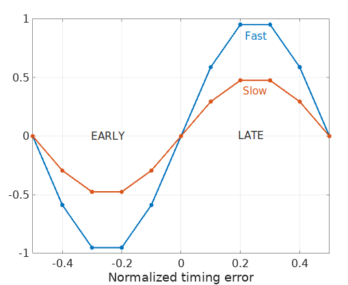
An S-curve gives us a control signal that can be used to adjust the timing. When we are late we want it to be positive so we can use it to hinder our clock accordingly, and likewise, we want it to be negative when we are early to use it to advance our clock. When we are synchronized we want its value to be as small as possible. Its slope at zero gives us an idea of how fast it can help us to synchronize. With a low slope it will take longer to synchronize. The next chart shows examples of two proverbial S-curves:
Let’s take a look now at what this transformation does to a GMSK signal. Here we have the differential phase of an AIS message with 9600 bauds, oversampled with T=10 and with a bit of noise added:

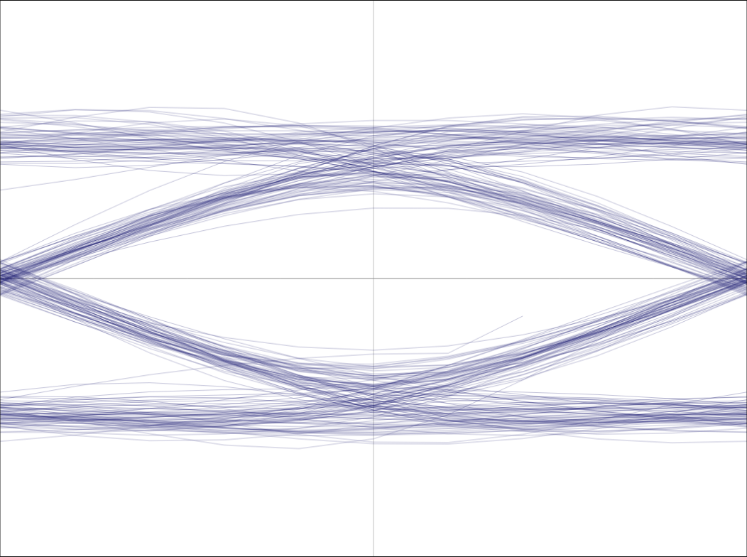
It’s a bit noisy but its eye diagram comes out well defined and it should not be a challenge for the clock recovery algorithm to work with it. This diagram has been prepared with the help from this simple interactive javascript tool.
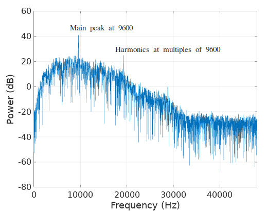
Surely enough, the spectrum of \(Re\{\dot{c}(t)\}\), the real component of the derivative of \(\tilde{c}(t)\), shows a strong peak at 9600, our symbol rate:
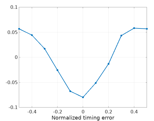
And its eye diagram shows the properties we are looking for in a S-curve:
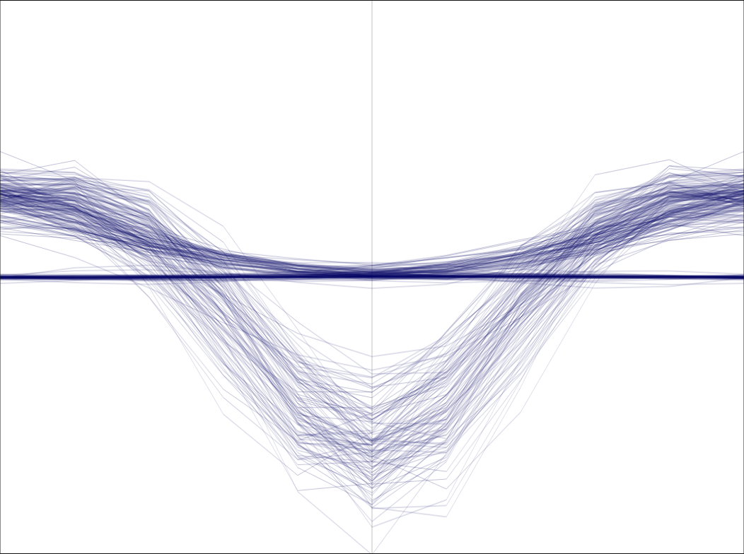
Notice however that this curve shows a bias of one quarter of the symbol period \(T\).
Average all the symbol periods from the eye diagram, the result (an approximation to its expected value) shows like this:

Which is a robust S-curve centered at about one quarter of the symbol period \(T\).
The most important detrimental effect to this method is the effect of series of consecutive symbol values in the data stream. Logically a long series of zeros or ones in the MSK signal produce a single tone frequency that doesn’t give any chance for the clock recovery. This is the reason why encoding schemas limit this effect by introducing “bit stuffing,” effectively breaking those long sequences by introducing alternating symbols in the data stream.
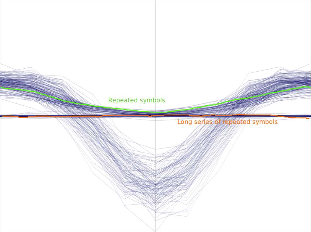
Moreover, the harmonics that showed up in the S-curve spectrum presented before are coming from those sequences of consecutive symbol values.
SNR analysis
Following a similar approach to Guobing et al in “Blind Frequency and Symbol Rate Estimation for MSK Signal under low SNR” we can estimate how is the SNR of D’Andrea’s fourth-order transformation in comparison to the original signal’s SNR.
Being of constant envelope, the power of an MSK signal goes with \(\dfrac{A^2}{2}\), where \(A\) is the amplitude of the signal. As far as the noise, we say its power is equal to the square of its standard deviation or \(\sigma^2\). Then, the power of our fourth order transformation:
\[\tilde{z}^2(t)\tilde{z}^{*2}(t-T) = (s(t)+n(t))^2(s(t-T)+n(t-T)^{*2}\]can be approximated, as far as power computation is concerned, by:
\[(\dfrac{A^2}{2})^4 + 4(\dfrac{A^2}{2})^3\sigma^2 + 6(\dfrac{A^2}{2})^2\sigma^4 + 4\dfrac{A^2}{2}\sigma^6 + \sigma^8\]The first term in the summation is our signal while the rest are its noise components. Normalizing \(\sigma\) to 1, the SNR of the original \(s(t)\) is then \(SNR(s) = \dfrac{A^2}{2}\) and the SNR of our fourth order transformation can be approximated by:
\[\dfrac{SNR(s)^4}{4SNR(s)^3 + 6SNR(s)^2 + 4SNR(s) + 1}\]We can see that this is about one fourth (6 dB less) for high SNR values of \(s(t)\) and it decreases rapidly for lower SNRs:
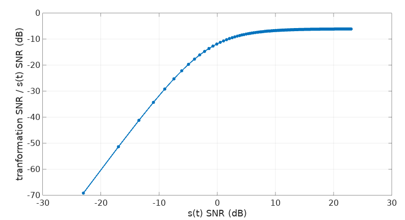
We can see then how the degradation of this transformation is worse in presence of noise in comparison to the original signal \(s(t)\). Still, it seems remarkably reliable, even when a considerable amount of noise is added to our original signal, to the point that its eye diagram starts to get all murky:
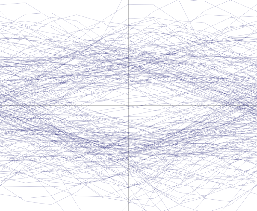
the averaged S-curve still holds its shape, although its amplitude has decreased:
Of course we are using here the whole signal (about 230 symbols) to average the S-curve. This approach might not be practical in some applications where low latency is critical.
Conclusion
This method shows great potential and an exploration of its limitations shows a number of avenues for further improvement:
A data-driven approach: given that some symbol repetitions are detrimental to the method, they can be detected and skipped from the clock recovery stage, or perhaps the S-curve coming from those repeated symbols can be manipulated to make it better behaved.
S-curve noise reduction: a number of different schemas can be applied to reduce the noise from the S-curve. The most immediate is to average values from a number of periods. The tradeoff here is that the longer our averaging, the more delay is added and the longer it will take for the method to synchronize, should this method be used for clock acquisition. An extended approach presented in some later papers by the same authors considered the autocorrelation also at multiples of \(T\), taking in consideration that the sign flips at even multiples.
I’ll leave it here for now.
Leave a Comment