
Signal Detection: Matched Filter
For burst-mode communications, where the signal of our interest is present in the communication channel for only a brief period of time, signal detection is the very first task in our receiver. This is opposed to continuous communications (e.g. broadcast radio or TV) where we can assume that the signal is present in the channel at all times and we can skip this stage.
Notice how our ability to detect the signal represents a ceiling to the overall receiver performance, often summarized in the packet error rate (PER) metric: a packet that we fail to detect is a packet that will never be recovered and therefore in error.
And to make things interesting, there is an engineering trade-off between a detection technique that is too lenient and has a high false alarm (false positive) probability versus another that is too strict and has a high miss detection probability.
For all these reasons signal detection is one of the most important tasks in our receiver and I think it’s worth it to dedicate this note to cover one of the most important techniques in this domain: matched filtering. If you have some experience with radio communications you probably know that this is the optimal technique in the presence of additive white Gaussian noise. You might even have gone through the math that proves this. Here I’m going to offer an approach that anybody with basic math skills can follow and use as a vehicle for the explanation, one more time, AIS communications.
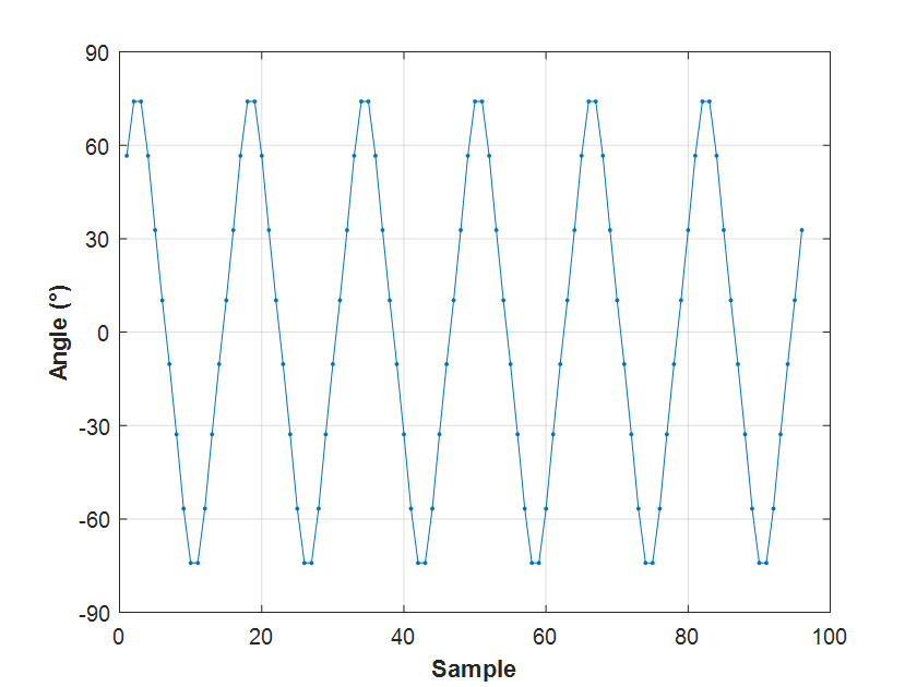
Checking the standard we find that all AIS messages start with a training sequence of 24 alternating 0’s and 1’s:
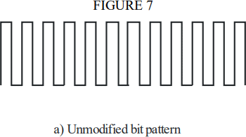
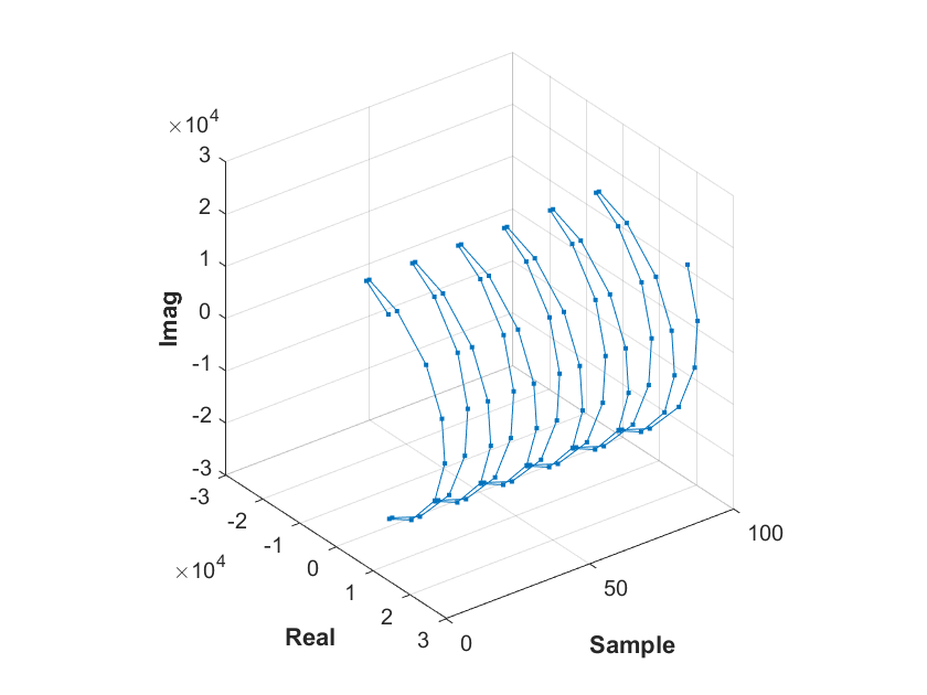
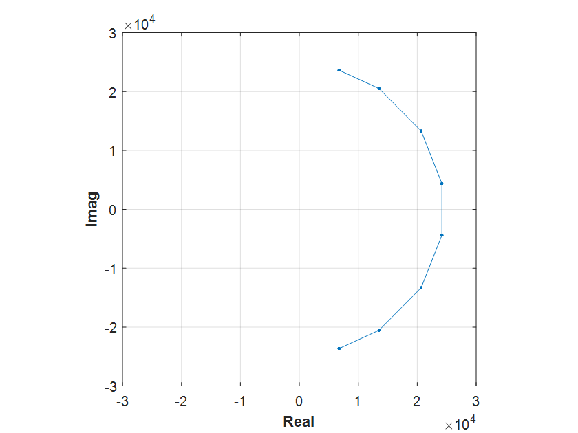
Once this sequence is converted to NRZI and passes through the GMSK modulator, which in this example we are going set to produce four samples per symbol, the 24*4 = 96 radio-frequency (RF) samples that are broadcasted take the following shape:
In matched filtering, the idea is pretty simple: convolve our incoming radio samples \(r_i\) with the conjugate of the training sequence samples \(m_i\):
\[y = \sum\limits_{n=1}^{N}{r_n m_n^*}\]where \(^*\) denotes complex conjugation and \(N\) is the number of samples in the training sequence, or 96 in our example. Notice by the way that the convolution result \(y\) is a complex number.
Without getting very deep in the equations, we can see that when \(r = m\) the effect of the multiplication consists of de-rotating all the samples placing them over the real axis. In polar notation, if \(m_n = \|m_n\| e^{i\phi_n}\), then
\[y = \sum\limits_{n=1}^{N}{m_n m_n^*} = \sum\limits_{n=1}^{N}{\|m_n\| e^{i\phi_n} \|m_n\| e^{-i\phi_n}} = \sum\limits_{n=1}^{N}{\|m_n\|^2}\]so \(\Re(y) = y\), equal to the energy of this sequence of samples, and \(\Im(y) = 0.\)
This technique is the optimal when the only signal impairment that we need to consider is AWGN. There are however a couple of impairments that unfortunately we can’t ignore in real life:
1. The carrier phase is unknown
This is typically indicated by saying that the original transmitted signal \(s\) has been rotated by an unknown phase \(\theta\):
\[r_n = s_n e^{i\theta}\]so our convolution becomes:
\[y = \sum\limits_{n=1}^{N}{s_n e^{i\theta} m_n^*} = e^{i\theta} \sum\limits_{n=1}^{N}{s_n m_n^*}\]Since \(\theta\) is unknown to the receiver it means that the convolution result \(y\) is a complex number pointing at a random angle. This is not the end of the world. What we can do is take its magnitude, or even better as we will see later, its squared magnitude:
\[\|y\|^2 = \|e^{i\theta}\sum\limits_{n=1}^{N}{s_n m_n^*}\|^2 = \|\sum\limits_{n=1}^{N}{s_n m_n^*}\|^2\]since
\[\|e^{i\theta}\| = 1\]To make this value useful as a detection score, we should not forget to normalize by the energies of our sequences, so the results remain invariant to the strength of the signal:
\[\text{detection score} = \frac{\|y\|^2}{\sum\limits_{n=1}^{N}{s_n s_n^*}\sum\limits_{n=1}^{N}{m_n m_n^*}} = \frac{\|\sum\limits_{n=1}^{N}{s_n m_n^*}\|^2}{\sum\limits_{n=1}^{N}{s_n s_n^*}\sum\limits_{n=1}^{N}{m_n m_n^*}}\] \[= \frac{\|\sum\limits_{n=1}^{N}{s_n m_n^*}\|^2}{\sum\limits_{n=1}^{N}{\|s_n\|^2}\sum\limits_{n=1}^{N}{\|m_n\|^2}} \tag{1}\label{eq:1}\]and since all the magnitudes are squared, we avoid computing square roots. Staying on the topic of implementation details and saving computations, notice that it makes a lot of sense to normalize in energy the \(m\) sequence beforehand.
To complete the picture, the following figure illustrates how the AIS training sequence matched filter detection score is affected by the signal quality:
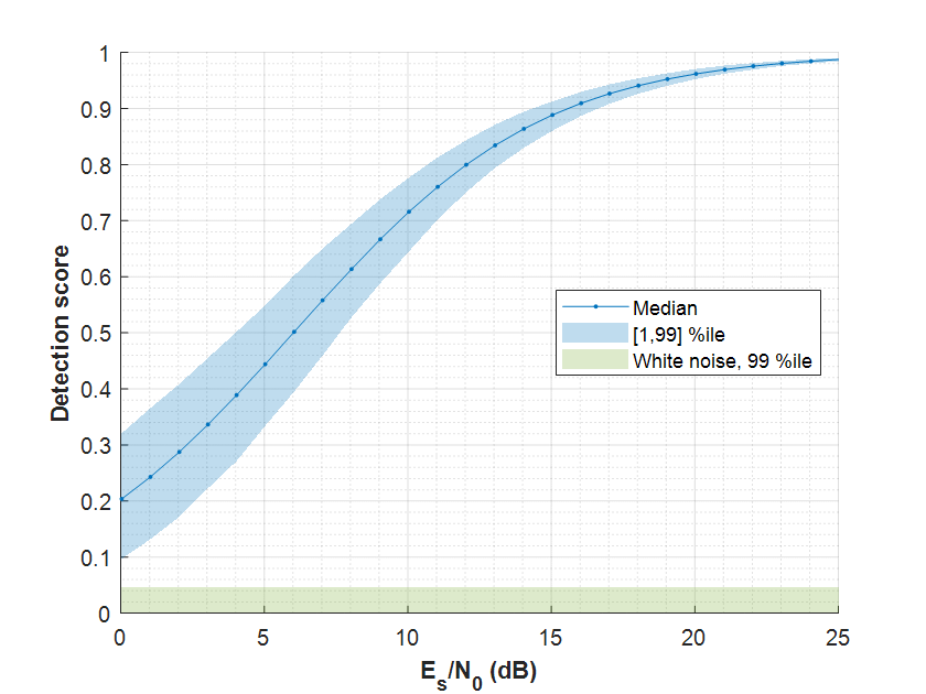
The maximum detection score is 1 for high quality signals and drops as the signal quality degrades. The appendix offers a qualitative analysis on this for anyone interested in digging deeper.
The blue band indicates the 1 to 99 percentile range. The green one is calculated from the detection scores when no signal, only white Gaussian noise, is present. We can see that by setting our detection score threshold to something about 0.07, we should be able to detect even very low quality AIS signals with a low probability of false detections. Please take note that this particular value is a design choice: you will need to check the values for your particular signal and decide what amount of false positives and missed detections you are comfortable with in your application.
All these considerations should prepared us to face up to the next challenge:
2. There is uncertainty with the signal frequency
We tell our AIS receiver to tune to the 162.025 MHz AIS channel 2 frequency and it tries, but it is never going to be at that exact frequency unless we work at NASA Deep Space Network and our radio uses an atomic clock to discipline its frequency reference. Our receiver might very well be a decent hobbyist SDR, mounting a ±1 ppm TCXO. We should then expect ±162 Hz of uncertainty at 162 MHz, which is small because, on the transmitting side, we find a transponder that, at best, follows the AIS specification mandating a carrier frequency error of ±500 Hz. Altogether, we have a frequency uncertainty of about ±700 Hz, which we can conservatively round to ±1 kHz.
What does this mean in terms of our ability to detect our signal? It means quite a lot for the matched filter technique. Using the AIS training sequence and applying a frequency offset, we can see how the detection score is affected:
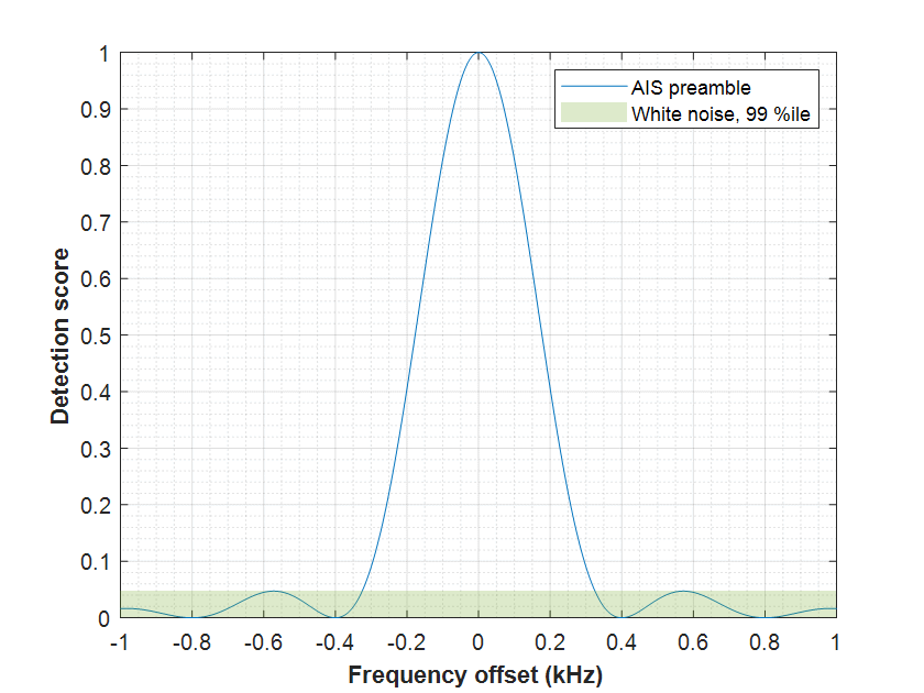
The score drops quickly and at ±300 Hz we are below the 99% percentile of white Gaussian noise. And this is without noise added to our signal. If we want to have enough margin we are going to be limited to maybe ±200 Hz, clearly insufficient for our ±1 kHz coverage requirement.
We have a couple of options at this point:
Brute force: saying that the unmodified matched filter detector is able to work in the range of ±200 Hz, we could have five of them running in parallel at frequencies 0, ±400 and ±800 Hz.
Try to be smart and exploit properties in the detection sequence. This is what I will propose for consideration on the next note.
Appendix
Shall we dare to explore how the detection score in the matched filter is affected by noise? Absolutely. Considering that the signal is affected by additive white Gaussian noise (AWGN), we have that \(s = m + w\). Our expression for the matched filter detection score is now:
\[\text{detection score} = \frac{\Bigl\|\sum\limits_{n=1}^{N}{(m_n + w_n)m_n^*}\Bigr\|^2}{\sum\limits_{n=1}^{N}{\|m_n + w_n\|^2}\sum\limits_{n=1}^{N}{\|m_n\|^2}}\] \[= \frac{\Bigl\|\sum\limits_{n=1}^{N}{m_n m_n^*} + \sum\limits_{n=1}^{N}{w_n m_n^*}\Bigr\|^2}{\sum\limits_{n=1}^{N}{\|m_n + w_n\|^2}\sum\limits_{n=1}^{N}{\|m_n\|^2}} = \frac{\Bigl\|\sum\limits_{n=1}^{N}{\|m_n\|^2} + \sum\limits_{n=1}^{N}{w_n m_n^*}\Bigr\|^2}{\sum\limits_{n=1}^{N}{(m_n + w_n)(m_n + w_n)^*}\sum\limits_{n=1}^{N}{\|m_n\|^2}}\] \[= \frac{\Bigl\|\sum\limits_{n=1}^{N}{\|m_n\|^2} + \sum\limits_{n=1}^{N}{w_n m_n^*}\Bigr\|^2}{\sum\limits_{n=1}^{N}{(m_n m_n^* + w_n m_n^* + m_n w_n^* + w_n w_n^*)}\sum\limits_{n=1}^{N}{\|m_n\|^2}}\] \[= \frac{\Bigl\|\sum\limits_{n=1}^{N}{\|m_n\|^2} + \sum\limits_{n=1}^{N}{w_n m_n^*}\Bigr\|^2}{\Bigl(\sum\limits_{n=1}^{N}{\|m_n\|^2} + \sum\limits_{n=1}^{N}{w_n m_n^*} + \sum\limits_{n=1}^{N}{m_n w_n^*} + \sum\limits_{n=1}^{N}{\|w_n\|^2}\Bigr)\sum\limits_{n=1}^{N}{\|m_n\|^2}}\]Reaching this point, we can note that the expected values of all the summations that involved cross \(w\) and \(m\) terms should be zero. This is because the expected value of summations of \(w\) should be zero by the definition of white noise and terms \(w m^*\) (or \(m w^*\)) are rotations and scaling that don’t change this property. Using a probabilistic approach we would say that this is true because, again by the definition of white noise, the noise \(w\) is uncorrelated with our sequence \(m\). Anyhow,
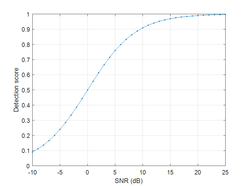
\[= \frac{\Bigl\|\sum\limits_{n=1}^{N}{\|m_n\|^2} + 0\Bigr\|^2}{\Bigl(\sum\limits_{n=1}^{N}{\|m_n\|^2} + 0 + 0 + \sum\limits_{n=1}^{N}{\|w_n\|^2}\Bigr)\sum\limits_{n=1}^{N}{\|m_n\|^2}}\] \[= \frac{\Bigl(\sum\limits_{n=1}^{N}{\|m_n\|^2}\Bigr)^2}{\Bigl(\sum\limits_{n=1}^{N}{\|m_n\|^2} + \sum\limits_{n=1}^{N}{\|w_n\|^2}\Bigr)\sum\limits_{n=1}^{N}{\|m_n\|^2}} = \frac{\sum\limits_{n=1}^{N}{\|m_n\|^2}}{\sum\limits_{n=1}^{N}{\|m_n\|^2} + \sum\limits_{n=1}^{N}{\|w_n\|^2}}\]The summations in \(m\) correspond to the energy of our signal in \(N\) samples and the summation in \(w\) is the energy of the noise in \(N\) samples as well. If we divide numerator and denominator by the energy of the noise we get our detection score in terms of our signal-to-noise ratio (SNR), since:
\[\frac{\sum\limits_{n=1}^{N}{\|m_n\|^2}}{\sum\limits_{n=1}^{N}{\|w_n\|^2}} = \text{SNR}\]so
\[\text{detection score} = \frac{\text{SNR}}{\text{SNR} + 1}\]Here \(\text{SNR}\) is in decimal scale, not in logarithmic (dB) scale. We see that when the SNR is very high the detection score should be close to 1. When signal and noise have the same power (SNR = 1 or 0 dB), the detection score drops to 0.5 and as the SNR drops, the detection score drops as well approaching 0:

Leave a Comment