
L&R Frequency Estimation
Estimating frequency deviations is a critical task in any modern communication device. Frequency deviations are inevitable. They come from inaccuracies in the oscillators at transmitter and receiver, aging of electronic components, Doppler effect when transmitter and/or receiver are moving.
The estimation those frequency deviations in real time is one of the main tasks of the “frequency tracking” module that you have probably seen in many communication system diagrams. To this purpose, some of the brightest minds in the field have dedicated countless hours of sleepless nights. Louise & Reggiannini (L&R in short) proposed in 1995 1 one of the smartest ways to estimate small frequency deviations in our carrier signal with high accuracy and low complexity. This method is still relevant almost 30 years later and the purpose of this note is to show how it works in enough detail that anyone with a minimal signal processing background should be able to understand.
Let’s jump into it.
Given a carrier signal (a single tone, if you prefer), we can define its \(k\) sample as:
\[\begin{equation} s_k = e^{j(2\pi f_n k + \theta_0)} \tag{1}\label{eq:1} \end{equation}\]where \(f_n = f_0/f_s\) is our carrier’s normalized frequency, with \(f_0\) being the actual carrier frequency and \(f_s\) our sampling frequency, and \(\theta_0\) an arbitrary initial phase. So far we are going to disregard the noise component but we keep in mind that noise mostly manifest as an additive component with Gaussian distribution (AWGN).
Similarly to many other methods for the estimation of a carrier frequency, L&R is based on auto-correlation properties. It’s going to be handy to use the following auto-correlation expression:
\[\begin{equation} R(k) \triangleq {\frac{1}{N-k}}\sum_{i=1}^{N-k} s_{i+k} s^{*}_{i} \tag{2}\label{eq:2} \end{equation}\]Where \(N\) is the number of samples that we have available for our analysis.
It’s not difficult to replace \eqref{eq:1} in \eqref{eq:2} to get, in the absence of noise, a very neat expression:
\[R(k) = {\frac{1}{N-k}} \sum_{i=1}^{N-k} e^{j(2 \pi f_{n} (i+k) + \theta_{0})} e^{-j(2 \pi f_{n} i + \theta_{0})} = e^{j 2 \pi f_{n} k}\](If you are not familiar with this, see appendix 1)
It says that the auto-correlation function \(R\) evaluated with a gap of \(k\) samples is equal to a phasor whose angle is \(2\pi k\) times our normalized carrier frequency. \(f_n\) can then be computed as:
\[f_n = {\frac{arg(R(k))}{2 \pi k}}\]And there we have a neat way to estimate our carrier frequency. There are however a couple of considerations at this point:
First, there are limits to the ranges of \(f_n\) we can detect. When \(2\pi k f_n\) exceeds the range \([-\pi, \pi]\) you have probably noticed we are going to have phase ambiguities that will confuse our results. In other words, we design our system to work with a maximum \(\lvert f_n \rvert\) and then our \(k\) is bounded by:
\[\begin{equation} k < {\frac{1}{2 \operatorname{max}(\lvert f_n \rvert)}} \tag{3}\label{eq:3} \end{equation}\]This explains the frequency tracking application. These auto-correlation frequency estimation methods are suitable to estimate small frequencies, and frequency deviations from the nominal are usually small in practical communications (if it’s large, you are probably getting a call from your friendly local RF spectrum regulator soon).
And a second consideration is, once we are convinced that this is a good idea and we want to implement it as the core of our frequency estimation module, which value of \(k\) should we use?
The answer from L&R is:
“Don’t take just one, take several. We are going to show you how the information from different \(R\) can be combined to produce a much better estimate while keeping the complexity low.”
Indeed, L&R explain how the problem of finding the optimal \(f_n\) estimate can be approximated as the solution of:
\[\operatorname{Im} \left\{ \sum_{i=1}^{N-k} k(N-k)R(k) e^{-j2\pi f_n k} \right\} = 0\](Details at appendix 2)
Note that this is not an approximation but the exact equation whose solution yields the best (“maximum-likelihood”) estimate that is possible to obtain from our \(N\) available samples.
As the authors explain, we can think of the \(k(N-k)\) factor the weights in a weighted average of our cross-correlation values. These weights make a parabola:
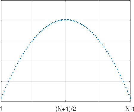
This makes a lot of sense. Intuitively, a small value of \(k\) is not ideal, since the frequency shift variation from one sample to the next is going to be drown in the noise. Are then larger values of \(k\) preferred…? After a large number or samples the frequency shift will be more visible, however, since the summation in \(R\) involves \(N-k\) elements, the larger \(k\), the fewer the number of elements we are going to add together (adding a large number of elements is intuitively good, because in the presence of uncorrelated noise, the noise component dampens out whereas the signal component reinforces). So very large values of \(k\) (near \(N\)) are also not ideal. As with many things in life the best is in the balance: values around \({\frac{N}{2}}\) come with the strongest weight.
In practice, the maximum \(k\) we can use is going to be determined by the maximum \(f_n\) we design for, as already stated in \eqref{eq:3}.
The L&R proposition at this point is:
- In order to limit the complexity of our implementation, compromise assuming that all the weights are constant and equal to \(1\). We will soon see how this works out.
- Limit the number of \(R(k)\) values that we compute to a given \(M\), with \(M \leq N-1\).
With these premises our maximum-likelihood equation simplifies to:
\[\operatorname{Im} \left\{ \sum_{i=1}^{M} R(k) e^{-j2\pi \hat{f_n} k} \right\} = 0\]The next assumption is key in reaching a viable estimator:
- Assume that \(2\pi f_n\) (the phase increment from sample to sample due to \(f_n\)) is small.
Then, remembering that for small angles \(cos(\theta) \approx 1\) and \(sin(\theta) \approx \theta\), our equation can be approximated by:
\[\operatorname{Im} \left\{ \sum_{i=1}^{M} R(k) (cos(-2\pi \hat{f_n} k) + j sin(-2\pi \hat{f_n} k)) \right\} \approx \operatorname{Im} \left\{ \sum_{i=1}^{M} R(k) (1 - j 2\pi \hat{f_n} k) \right\} = 0\]Minding that our \(R(k)\) are a complex values and that \(\operatorname{Im} \{(a+jb)(1-jc)\} = b-jac\), we get:
\[\sum_{i=1}^{M} \operatorname{Im} \{R(k)\} - \sum_{i=1}^{M} \operatorname{Re} \{R(k)\} 2\pi \hat{f_n} k = 0\]and therefore
\[\hat{f_n} = {\frac{\sum_{i=1}^{M} \operatorname{Im} \{R(k)\}} {2\pi \sum_{i=1}^{M} k \operatorname{Re} \{R(k)\}}}\]So far so good, but at this point we are going to diverge from the original L&R paper. I haven’t been able to find my way around the next step. According to the paper, and without introducing more assumptions, L&R claim that:
\[\sum_{i=1}^{M} \operatorname{Im} \{R(k)\} \approx M \operatorname{arg} \left\{ \sum_{i=1}^{M} R(k) \right\}\] \[\sum_{i=1}^{M} k \operatorname{Re} \{R(k)\} \approx {\frac{M(M+1)}{2}}\]I’m probably making some mistakes because my numerical simulations don’t agree with this. I’d be happy to get a second opinion from anybody…
However, I’m also happy that resorting to geometry, it’s possible to make progress and actually reach the same conclusion as L&R.
Going back to our \(R(k)\) definition, when applied to a pure noiseless carrier we have seen that it simplifies to
\[R(k) = e^{j 2 \pi f_n k}\]Taking \(k \in [1,M]\), we see its representation is a “train” of phasors around the unit circumference separated by an angle \(\theta = 2 \pi f_n\):
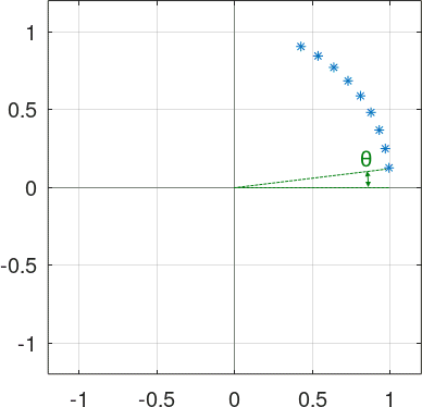
If we rotate this train clock-wise by \({\frac{M+1}{2}}\theta\), the figure becomes symmetrical around the \(X\) axis:
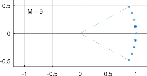

regardless of whether \(M\) is even or odd.
It’s now easy to get the intuition that the sum of the \(M\) real components of these rotated \(R(k)\) can be approximated by \(M\), given that the angle \(\theta\) is small, and that the sum of the imaginary components is going to cancel out (that interestingly true even if the angle is not so small).
In other words we are saying that
\[\sum_{i=1}^{M} R(k) e^{-j 2 \pi {\frac{M+1}{2}} f_n} \approx M\]or
\[\sum_{i=1}^{M} R(k) \approx M e^{j 2 \pi {\frac{M+1}{2}} f_n}\]taking the angle of both sides
\[\operatorname{arg} \left\{ \sum_{i=1}^{M} R(k) \right\} \approx 2 \pi {\frac{M+1}{2}} f_n\]so, our \(f_n\) can be approximated by
\[\hat{f_n} = {\frac{1}{\pi(M+1)}} \operatorname{arg} \left\{ \sum_{i=1}^{M} R(k) \right\}\]which is the final form of the L&R estimator.
It’s probably a good idea to let the reader at this point take a deserved rest, leaving some additional thoughts on the L&R frequency estimation method for a later note.
Appendix 1
Replacing
\[s_k = e^{j(2\pi f_n k + \theta_0)}\]in
\[R(k) \triangleq {\frac{1}{N-k}}\sum_{i=1}^{N-k} s_{i+k} s^{*}_{i}\]yields
\[R(k) = {\frac{1}{N-k}} \sum_{i=1}^{N-k} e^{j(2 \pi f_{n} (i+k) + \theta_{0})} e^{-j(2 \pi f_{n} i + \theta_{0})}\] \[= {\frac{1}{N-k}} \sum_{i=1}^{N-k} e^{j(2 \pi f_{n} (i+k) + \theta_{0} - 2 \pi f_{n} i - \theta_{0})} = {\frac{1}{N-k}} \sum_{i=1}^{N-k} e^{j 2 \pi f_{n} k}\] \[= {\frac{e^{j 2 \pi f_{n} k}}{N-k}} \sum_{i=1}^{N-k} 1 = {\frac{e^{j 2 \pi f_{n} k}}{N-k}} (N-k)\] \[= e^{j 2 \pi f_{n} k}\]Appendix 2
OK, this is a bit involved but not difficult. First of all, a reminder of the maximum-likelihood frequency estimation formula:
\[\begin{equation} \mathit{ML}(x) = \sum_{k=1}^{N} \sum_{m=1}^{N} s_k s_m^* e^{-j 2 \pi x (k-m)} \tag{4}\label{eq:a21} \end{equation}\] \[\DeclareMathOperator*{\argmax}{argmax} \hat{f_n} = \argmax_{x} \mathit{ML}(x)\]In words, our best possible estimate \(\hat{f_n}\) is the one that maximizes the sum of all the possible cross products between our samples, counter-rotated by a factor of the number of samples there are in between. We can see why this makes sense by repeating the same exercise as in appendix 1:
\[\mathit{ML}(f_n) = \sum_{k=1}^{N} \sum_{m=1}^{N} e^{j 2 \pi f_n k} e^{-j 2 \pi f_n m} e^{-j 2 \pi f_n (k-m)} = \sum_{k=1}^{N} \sum_{m=1}^{N} 1 = N^2\]The value of \(\mathit{ML}(x)\) will be lower than \(N^2\) for any other value of \(x\). This is also true in the presence of AWGN.
The maximum of \eqref{eq:a21} happens at an \(x\) such that it makes zero the partial derivative with respect to \(x\), and since \({\frac{d(e^{ax})}{dx}} = a e^{ax}\), we get the equation:
\[\sum_{k=1}^{N} \sum_{m=1}^{N} -j 2 \pi (k-m)s_k s_m^* e^{-j 2 \pi x (k-m)} = 0\]and getting rid of the \(-j 2 \pi\) factor:
\[\sum_{k=1}^{N} \sum_{m=1}^{N} (k-m)s_k s_m^* e^{-j 2 \pi x (k-m)} = 0\]We should note that we are adding together \(N \times N\) elements and that we get zeros whenever \(k = m\), or along the main diagonal if it was a matrix:
\[\begin{equation} \left[ {\begin{array}{cccc} 0 & -s_1 s_2^{*} e^{j 2 \pi x} & \cdots & -(N-1) s_1 s_N^{*} e^{j 2 \pi x (N-1)}\\ s_2 s_1^{*} e^{-j 2 \pi x} & 0 & \cdots & -(N-2) s_2 s_N^{*} e^{j 2 \pi x (N-2)}\\ \vdots & \vdots & \ddots & \vdots\\ (N-1) s_N s_1^{*} e^{-j 2 \pi x (N-1)} & (N-2) s_N s_2^{*} e^{-j 2 \pi x (N-2)} & \cdots & 0\\ \end{array} } \right] \tag{5}\label{eq:a22} \end{equation}\]and the symmetry between the upper and lower triangular sections is now exposed as an opportunity to exploit. Our double summation is then equivalent to:
\[\sum_{k=2}^{N} \sum_{m=1}^{k-1} \left( (k-m)s_k s_m^* e^{-j 2 \pi x (k-m)} - (k-m)s_m s_k^* e^{j 2 \pi x (k-m)} \right) = 0\]and since
\(a b^{*} e^{-jc} - a^{*} b e^{jc} = a b^{*} e^{-jc} - ( a^{*} b e^{jc})^{*}\) and \(d - d^{*} = 2j \operatorname{Im} \left\{ d \right\}\), our equation is simplified to
\[\sum_{k=2}^{N} \sum_{m=1}^{k-1} 2j \operatorname{Im} \left\{ (k-m)s_k s_m^* e^{-j 2 \pi x (k-m)} \right\} = 0\]Now, with the help of paper and pencil, it can be seen that the following summations produce identical terms: instead of iterating over rows and columns, we are iterating here through the diagonals of the lower triangular section of the matrix in \eqref{eq:a22}.
\[\sum_{k=1}^{N-1} \sum_{i=1}^{N-k} 2j \operatorname{Im} \left\{ k s_{i+k} s_i^* e^{-j 2 \pi x k} \right\} = 0\]which equivalent to
\[\operatorname{Im} \left\{ \sum_{k=1}^{N-1} k \sum_{i=1}^{N-k} s_{i+k} s_i^* e^{-j 2 \pi x k} \right\} = 0\]which we can express in terms of our cross-correlation function \(R(k) = {\frac{1}{N-k}}\sum_{i=1}^{N-k} s_{i+k} s^{*}_{i}\), yielding the final form of our equation:
\[\operatorname{Im} \left\{ \sum_{i=1}^{N-k} k(N-k)R(k) e^{j-2\pi f_n k} \right\} = 0\]References
M. Luise and R. Reggiannini, “Carrier frequency recovery in all-digital modems for burst-mode transmissions,” in IEEE Transactions on Communications, vol. 43, no. 2/3/4, pp. 1169-1178, Feb./March/April 1995, doi: 10.1109/26.380149. ↩
Leave a Comment