RF Direction Finding, Adcock/Watson-Watt Technique (III)

Imagine a country road somewhere in the UK. A black and grey Daimler dashes in the middle of the night. Inside, a young Winston Churchill is being driven to an undisclosed air field for the demonstration of a new technology that is going to revolutionize warfare. WWI is already over but the echoes of an incoming thunderstorm are there for anybody who cares to listen. Inside the hangar, Robert Watson-Watt and his team are getting ready. An airplane is already flying several kilometers away, equipped with a radio transmitter. The purpose of this device, Robert explains, is to detect the direction of the transmitter, and hence, the plane:

– We are going to see in a minute a line of light drawn on this circular screen. The angle of the line corresponds with the direction of the radio transmitter. As the plane moves from left to right, we are going to see how this angle changes.

– Fascinating…

– The radio frequency signal that is captured by the antenna poles you have seen outside is being manipulated in a way that alters the electric fields on the horizontal and vertical plates of this device, we call it “oscilloscope.”

– These are all new toys you have here…

– Yes, this is all state-of-the-art. Those plates I was talking about modify the direction of the electrons emitted by the cathode-ray tube behind the screen. When the electrons hit the green phosphor screen, we see a bright line with an inclination that follows the angle of arrival of the incoming radio frequency signal.

– Only the angle of arrival? How about the distance?

– We are working on that sir, it might be ready for a demonstration soon. We are calling it “radar.”

Fast-forward about 100 years later, we are not going to implement the Watson-Watt (WW) direction finding technique, which has been the object of the last couple of articles, using an analog oscilloscope. Most likely we are going to use some kind of SDR where the bulk of the signal “manipulation” is executed in the digital domain by some sort of computing device.

The object of this last article in the series is to give some implementation “tricks” and practical notes. Let’s get to it.

Implementation notes

We must start remembering one more time the foundational equations of this technique:

\(\phi\) is our seeked angle of arrival and \(r_{NS}\), \(r_{EW}\) and \(r_O\) are the three outputs coming out of our Adcock antenna.

Trick #1: Sign of phase difference

This is how the “sign of the phase difference” between two vectors can be computed easily. Remember that \(r_{NS}\) and \(r_{EW}\) should only be at either + or - 90° with respect to \(r_O\):

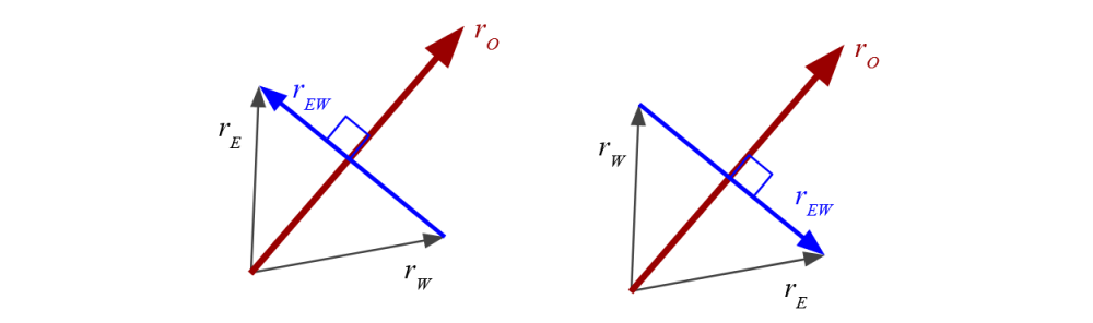
So, the sine of the angle between those two vectors should be +1 when they make +90° and -1 when they make -90°. Taking into account that we are going to have some added noise, we can say that when the sine of the angle between those two vectors is positive, we consider the sign as +1 and when negative, -1. Now, the sign of the sine of the angle between two vectors can be computed very simply. Given two vectors:

then

and since \(A\) and \(B\) are positive magnitudes we can say that

which can be computed with two multiplications and one comparison.

Trick #2: Computation of atan2

We compute \(atan2(y,x)\) using a table. The signs of \(x\) and \(y\) will tell us the quadrant and the ratio \(y/x\) will tell us the degrees inside the quadrant. Since the accuracy of the WW technique is going to be worse than 1 degree, we don’t really need a very big table. One more consideration here is that our \(x\) and \(y\) are magnitudes. Magnitude of \(x\) is computed as \(\sqrt{\Re(x)^2+\Im(x)^2}\). We can skip computing expensive square roots by making our table be a table of \(atan2(\sqrt{y2},\sqrt{x2})\) where \(x2\) and \(y2\) are our squared magnitudes.

Trick #3: Averaging

To reduce the noise in our estimates we can average results over a period of time. I think I’ve mentioned this before: you can’t average angles just like that. Results in degrees that are very close like [0, 359, 1, 358, 2] are going to be averaged to something around 180° which is obviously wrong. What you want to do is to average the \(x\) and \(y\) values, the arguments to your \(atan2\) computation. Then, once you have accumulated enough values, compute the \(atan2\) of the averaged \(x\) and \(y\).

If we want to get an idea of how noisy our angle of arrival estimates are, we can compute their circular standard deviation.

Trick #4: You can work in the frequency domain

If we understand the Fourier transform applied to our input signal as a linear decomposition in their frequency components, then the same WW formulas apply in the frequency domain. This knowledge can give us a significant advantage. Being our signal of interest a narrow-band signal, with most of its energy focused on a few frequency bins, we can compute \(R_O\), \(R_{EW}\) and \(R_{NS}\) as the Fourier-transformed versions of our input signals \(r_O\), \(r_{EW}\), \(r_{NS}\) and then we can proceed with our angle of arrival computations with just the frequency bins that correspond to our signal. This would be equivalent to applying a narrow band pass filter and then working in the time domain, but the cool thing of working in the frequency domain is that, if your SDR processor can afford it, you can compute the angle of arrival for each frequency bin. If you do this continuously and assign colors to the angles, you can get something like this:

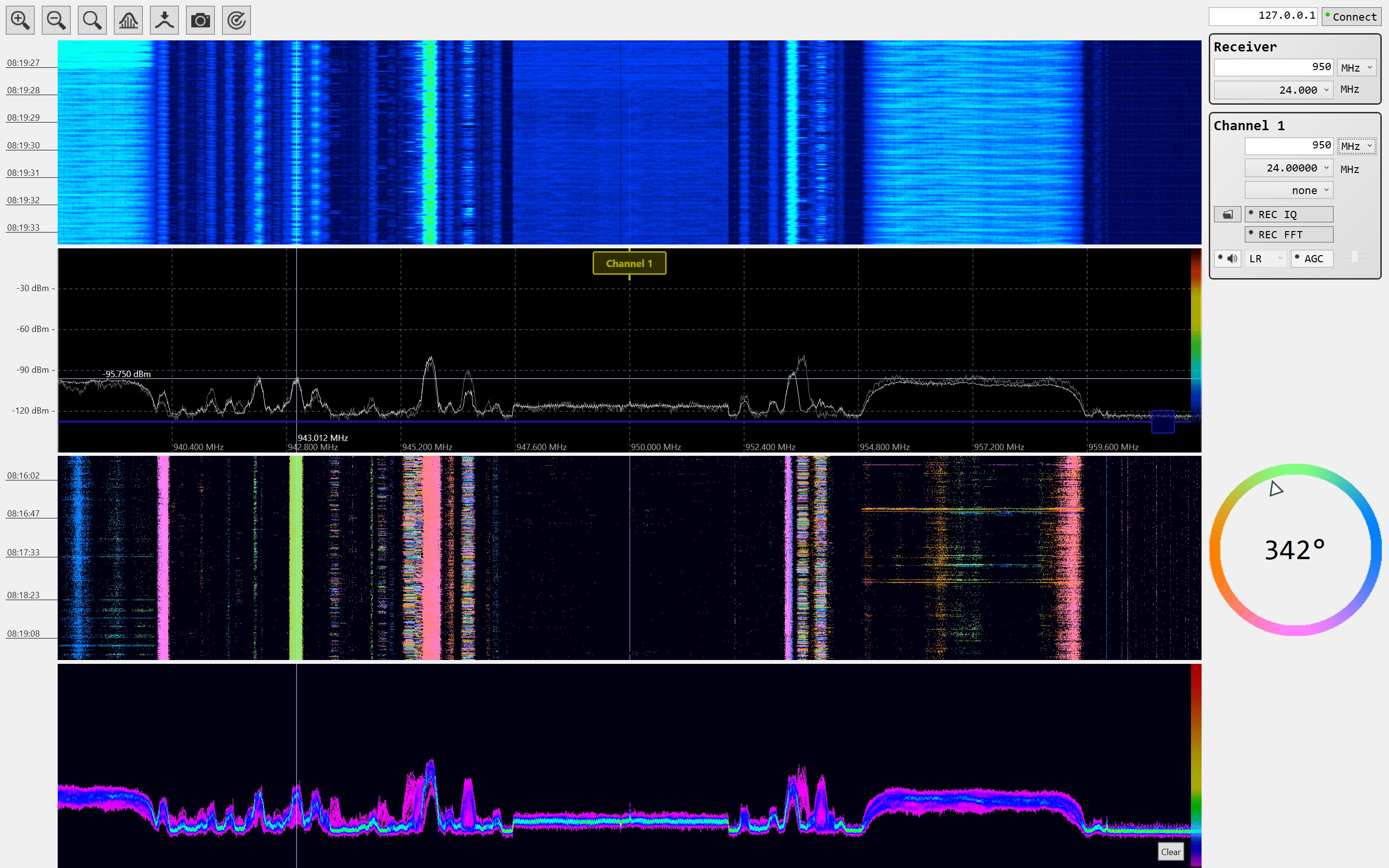
This is an improvement over the green phosphor screen of Sir Robert Watson-Watt. The third panel from the top shows in real time the angle of arrival of the different radio signals inside the receiver’s bandwidth. The horizontal axis is frequency, time in the vertical and the color wheel at the right gives the mapping between color to angle of arrival.

This is all I have on this topic. Cheers!