Frequency Shifting

This time I’m going to analyze some common frequency shifting techniques, particularly fixed-point implementations that are more challenging and where compromises need to be made between accuracy and computing performance.

Frequency shifting is a building block in the body of signal processing. Its purpose is straightforward: translate in frequency an input signal. This is commonly used in radio applications where a given signal that shows at some offset from our tuning frequency needs to be “base banded” (translated to 0 frequency) for further processing. Other applications include the correction of frequency deviations, maybe coming from a Doppler effect when the transmitter and/or receiver are not static or coming from inaccuracies in the local oscillators of transmitter and/or receiver.

Thanks to Euler the operation of frequency shifting can be expressed as a one-liner:

where \(s(t)\) is our original signal, \(s'(t)\) is its frequency shifted version and \(f_\Delta\) is the desired frequency shift in Hz. Frequency shifting is just the multiplication of our original signal with a phasor rotating at a frequency equal to the desired shift.

This is demonstrated easily. Thanks to Fourier we know that any signal (at least any for our engineering purposes) can be represented as a linear combination of its frequency components:

therefore, a multiplication by the phasor \(e^{j 2 \pi f_\Delta t}\) produces a frequency shifting to all its frequency components by \(f_\Delta\) Hz:

The digital implementation of a frequency shift is then pretty straightforward. It requires the generation of a phasor at our desired frequency shift with magnitude 1 (unless we want to modify the amplitude of the input signal) and perform a complex multiplication sample by sample of the original signal with this phasor.

To take into account that in the digital domain, since we are sampling our signal at some sampling frequency \(f_s\), the frequency shift would need to get normalized by this frequency. So, to achieve a frequency shift of \(f_\Delta\) at \(f_s\) sampling rate, our phasor needs to run at \(f_\Delta/f_s\) Hz.

Pre-computed table

There are many different ways to produce this phasor, one option is to use a pre-computed table. We know that the phasor will repeat at integer multiples of \(f_\Delta / f_s\). To give a numeric example, let’s say that our sampling frequency is 96 kHz and we want to do a frequency shift by 3 kHz. In this lucky case we only need a table to hold 32 samples for our phasor since it will repeat after so many samples. We are lucky because our shift frequency is an integer multiple of our sampling frequency: 96000/3000 = 32. In other cases we won’t be so lucky, for instance, for a desired frequency shift of 3001 Hz the size of the required table is going to be 3001*96000 = 28809600, which might be prohibitively large for our application. In general the size of the table is given by the expression:

Where GCD stands for “greatest common divisor.” The expression also takes into account that the frequency shift can be a negative value.

In practice there is not much difference between a frequency shift of 3000 or 3001 Hz, so if we go down this road we can compromise with accuracy and find a value that is close enough to our desired one that can give us a reasonable table size. It helps a lot if we have the liberty of choosing a sampling frequency that give us many factorization options (I’m thinking of a sampling frequency that can be expressed as \(2^a 3^b 5^c\) where a, b and c are integers). For sure we don’t want to choose a prime number neither for our sampling nor shifting frequencies.

On-the-fly

Computing our phasor on the fly can be a reasonable alternative to the table approach. Thanks again to Euler we know that a phasor at frequency \(f_\Delta/f_s\) can be generated by a recurrent expression:

phasor[0] = 1

phasor[i] = phasor[i-1]\((cos(2 \pi f_\Delta/f_s)+j sin(2 \pi f_\Delta/f_s))\)

So, we only need one complex multiplication per sample and we avoid altogether the need for any pre-computed table. A complex multiplication can be implemented with four scalar multiplications plus two additions. In some CPU architectures (I’m thinking SIMD) this can be accomplished with ease and might be better performing than a table implementation since we avoid memory accesses and cache misses. However there is a caveat here. It shows quite dramatically in a typical fixed-point implementation like this one:

#include <iostream>
#include <complex>

int16_t to_int16(int32_t v) {

    // Saturate to the [-32768, 32767] range
    return (v > 32767)? 32767 : (v < -32768)? -32768 : (int16_t)v;
}

int16_t to_int16(float v) {

    v = roundf(v);
    // Saturate to the [-32768, 32767] range
    return (v > 32767.0f)? 32767 : (v < -32768.0f)? -32768 : (int16_t)v;
}

std::complex<int16_t> multiply_i16(const std::complex<int16_t>& a,
                                   const std::complex<int16_t>& b) {

    // Perform the computation in 32 bits
    int32_t re_a = std::real(a);
    int32_t im_a = std::imag(a);
    int32_t re_b = std::real(b);
    int32_t im_b = std::imag(b);

    int32_t re_c = re_a*re_b - im_a*im_b;
    int32_t im_c = re_a*im_b + im_a*re_b;

    // Scale down back to 16 bits
    return std::complex<int16_t>(to_int16(re_c >> 15),
                                 to_int16(im_c >> 15));
}

float fs = 96000.0f;
float fd =  3000.0f;

// We enjoy the luxury of a more accurate floating-point
// phase_per_sample computation
float rads_per_sample = 2.0f*M_PI*fd/fs;
std::complex<int16_t> phase_per_sample(to_int16(cosf(rads_per_sample)*32768.0f),
                                       to_int16(sinf(rads_per_sample)*32768.0f));

std::cout << "Phase per sample: " << phase_per_sample << std::endl;

std::complex<int16_t> phasor(32767, 0);

void frequency_shift(const std::complex<int16_t>* input_signal,
                     std::complex<int16_t>* output_signal,
                     unsigned int n_samples)
{
    for (unsigned int i=0; i < n_samples; i++) {
        // Rotate the input signal
        output_signal[i] = multiply_i16(input signal[i], phasor);

        // Rotate our phasor
        phasor = multiply_i16(phasor, phase_per_sample);
    }
}

The values are 16-bit integers in the range [-32768,32767] (I believe this is called “1.15 format”) and are scaled up to fully utilize the available dynamic range. The complex multiplication is performed in 32-bits and scaled down so the results go back to the 16-bit range.

Plotting the magnitude of the generated phasor exposes the problem:

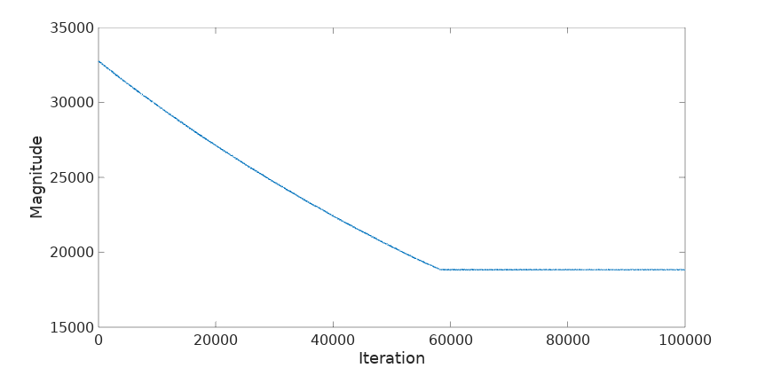
The magnitude keeps dropping until, by the quirkiness of fixed-point arithmetics, it reaches a stability point at around 18839 or back to floating-point at 18839/32768 = 0.57. That means that if we use this phasor to frequency-shift our signal, we are going to be attenuating it by that much, something not acceptable in most applications.

There are a number of ways to overcome this problem. One of them we can find in GNU Radio’s rotator:

gr_complex rotate(gr_complex in)
{
    d_counter++;

    gr_complex z = in * d_phase;    // rotate in by phase
    d_phase *= d_phase_incr;        // incr our phase (complex mult == add phases)

    if((d_counter % 512) == 0)
        d_phase /= std::abs(d_phase);     // Normalize to ensure multiplication is rotation

    return z;
}

After a number of iterations (512) the magnitude of the phasor is set back to 1. Why not do this adjustment at every iteration? Well, behind the innocent looking std::abs there is a square root lurking, which is computationally expensive (and a headache in a fixed-point implementation).

But there is one more reason to frown upon this implementation: the periodic adjustment we introduce in our phasor is going to inevitably produce some harmonics, detrimental to its purity. Let’s see this next with a modified version of the previous fixed-point code that includes the GNU Radio’s rotator magnitude compensation logic:

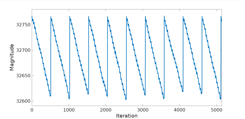
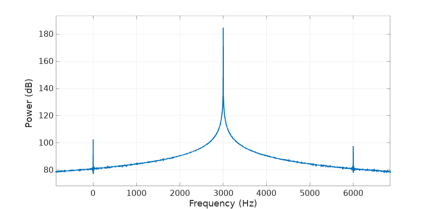
As expected the compensation kicks in every 512 samples bringing the magnitude back to nominal. The mean magnitude is 32688.45 and its standard deviation 45.89. Not bad, but the saw-tooth envelope is going to show up in the phasor’s FFT:

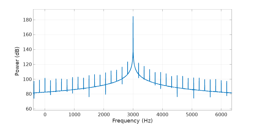
Sure enough, it shows as harmonics of 96000/512 or 187.5 Hz centered around the 3000 Hz phasor main frequency.

Proposal for an alternative fixed-point implementation

Let’s see if we can do better than this, both in terms of signal quality and computation complexity. First of all we need to understand why the phasor is decreasing its magnitude with each iteration. The reason is because phase_per_sample in the example code is 32138+j639 (let’s call this value \(p_0\)). It has a magnitude \(m_0 \approx\) 32767.69, a bit short of 32768. This difference, even small, is going to accumulate after each iteration, producing an exponential effect. At iteration \(n\) the attenuation factor is going to be \((m_0-32768)^n\). We can try to increase a bit the magnitude of this value, using a phase_per_sample of 32139+j6393 (\(p_1\)), with a magnitude \(m_1 \approx\) 32768.67, a bit higher than 32768, introducing a gain of \((m_1-32768)^n\) with each iteration. Fixed-point lack of accuracy is not working out well for us. In fact the only possible phase_per_sample values that produce an exact magnitude of 32768 in 16-bit arithmetic are the trivial -32768 (corresponding to a frequency shift of \(\pm f_s/2\)) and -j32768 (frequency shift of \(3 f_s/4\), equivalent to \(- f_s/4\)).

The trick I’m proposing here is to play with these two values \(p_0\) and \(p_1\), one that is a notch below the ideal magnitude of 32768 and one that is a notch above it. We are going to detect the magnitude of the phasor at each iteration (we don’t need to compute the square root, the squared magnitude would do) and, in some sort of closed-loop control system, we are going to use \(p_1\) when the magnitude is lower than the ideal and \(p_0\) the other way around.

The code would look like this:

...

std::complex<int16_t> phasor(32767, 0);
std::complex<int16_t> p0 = ... // Compute p_0, with magnitude slightly smaller than 32768
std::complex<int16_t> p1 = ... // Compute p_1, with magnitude slightly bigger than 32768

void frequency_shift(const std::complex<int16_t>* input_signal,
                     std::complex<int16_t>* output_signal,
                     unsigned int n_samples)
{
    for (unsigned int i=0; i < n_samples; i++) {
        // Rotate the input signal
        output_signal[i] = multiply_i16(input signal[i], phasor);

        // Rotate our phasor
        std::complex<int16_t> phase_per_sample;
        {
            // Calculate the squared magnitude of the phasor
            int32_t x = (int32_t)std::real(phasor);
            int32_t y = (int32_t)std::imag(phasor);
            int32_t m = x*x + y*y;
            if (m > 32768*32768) {
                phase_per_sample = p0; // Too big, use the small one
            } else {
                phase_per_sample = p1; // Too small, use the big one
            }
        }
        phasor = multiply_i16(phasor, phase_per_sample);
    }
}

The mean magnitude in this case is 32769.05 and standard deviation 1.68. Really good, but what’s even better is how this phasor looks in the frequency domain:

It’s almost as good as it can get taking into account the unavoidable quantization errors in a fixed-point implementation.

Notes

First notice that this proposed implementation requires the computation of the squared magnitude of the phasor with each iteration, at a cost of two multiplications, one addition and one more comparison to decide between the two pre-computed phase-per-sample values. If this is too expensive for our hardware we can fall in the temptation of adjusting the phasor not every sample but every n samples. This will affect the quality of our signal with the introduction of harmonics at \(f_s/n\) as shown for the GNU Radio’s rotator.

Second, this implementation fails to work for shifts very close to 0 or \(+f_s/4\). The reason is because these frequency shifts produce a \(p_0 =\) 32767 and \(p_0 =\) j 32767 respectively. In these cases we can’t find their corresponding \(p_1\) with a magnitude slightly larger than 32768 since we are already at the end of the representable 16-bit range. Unfortunately those cases will need to be handled individually. When \(f_\Delta\) is near 0 we can round it to 0 and just do the best thing there is to be done in DSP: nothing. On the other hand, frequency shifts close to \(+f_s/4\) can be rounded to exactly one quarter of \(f_s\), which can be implemented with just additions and substractions of the real and complex components of the input signal avoiding multiplications all together (see Digital Signal Processing Tricks - Frequency Translation without multiplication by Richard Lyons).

And third, there is a bit of inaccuracy to the frequency shift. In our case the \(p_0 =\) 32138+j6393 and \(p_1 =\) 32139+j6393 correspond exactly to frequency shifts equal to 3000.16 and 3000.07 Hz respectively, using the formula \(\dfrac{f_s}{2\pi}atan2(imag(p), real(p))\). If this inaccuracy is not acceptable then we can apply some frequency correction to the phasor but again minding that periodic corrections are going to introduce harmonics in our phasor.