Frequency Estimation

There is something on the last article, concerned with frequency shifting, that called my attention while I was preparing it. I was showing there a synthesized phasor in the frequency domain, something that can be produced with the following Octave code:

    % FFT plotting, with thanks to Jason R
    % https://dsp.stackexchange.com/questions/2970/how-to-make-frequency-axis-for-even-and-odd-fft-length
    function plot_fft(s, fs);
        n=numel(s);
        df = fs/n;
        ff = (0:(n-1))*df;
        ff(ff >= fs/2) = ff(ff >= fs/2) - fs;
        plot(fftshift(ff), 20*log10((abs(fftshift(fft(s))))/n), '*-');
    end

    t = (0:999);
    f = 12345;
    fs = 96000;
    s=cos(2*pi*t*f/fs) + i*sin(2*pi*t*f/fs);
    plot_fft(s, fs);

which produces the following figure: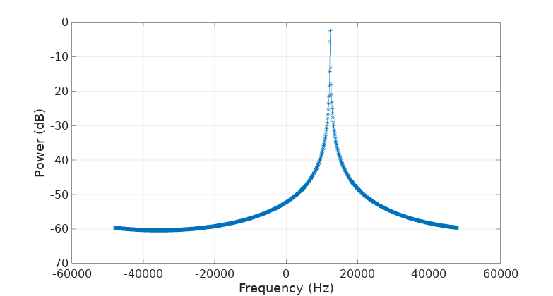

but… is this correct? Shouldn’t a phasor produce a single “line” spectrum, with all its energy focused in one single frequency bin?

Surely the problem is that I forgot again to “window” the signal, one of DSP’s capital sins:

    ws = s .* hamming(numel(s));
    plot_fft(ws,fs);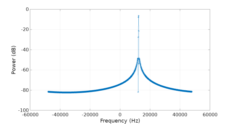

Nope, this is still not good… Actually the Wikipedia’s article on window functions does a good job at explaining what’s going on. The problem is that the Fourier transform (as well as the DFT used here) assumes that the signal is periodic. A phasor is indeed periodic, however the period in sample units of our phasor is, as described in the mentioned frequency shifting article:

which in our case is 5267200 samples. We are presenting 1000 samples instead to the DFT, so from the point of view of the DFT we are presenting a non-periodic set of samples. The discontinuity between one period to the next is producing the “spectrum leakage” to the neighbor frequency bins.

For confirmation, let’s see what happens if we present to the DFT the exact number of samples that makes our set truly periodic:

    t = (0:f*fs/(gcd(f,fs)^2)-1);
    ...
    % Notice that we are not using a window function:
    plot_fft(s,fs);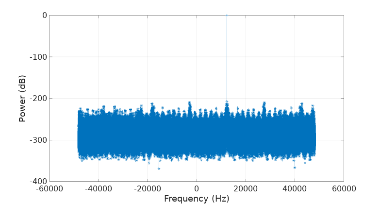

Bingo, no leakage whatsoever as it should be and no need to “window” our signal either. Take those -200 dB values from the plot as zero power since that’s pretty much the resolution of our floating point computation.

Being presented with a phasor of unknown frequency (a carrier signal for instance), if we were able to estimate its frequency (and therefore its period), then we should be able to produce an undistorted representation of our signal in the frequency domain by presenting the DFT with the appropriate number of samples corresponding with our signal’s period and we won’t need to apply any window function to them beforehand. This high magic is called coherent sampling.

There is a caveat, as there always is. This coherent sampling is unmerciful to inaccuracies in the estimation of our signal’s period. Let’s say we are short of one sample (out of 5267200!):

    t = (0:f*fs/(gcd(f,fs)^2)-1 -1);
    ...
    plot_fft(s,fs);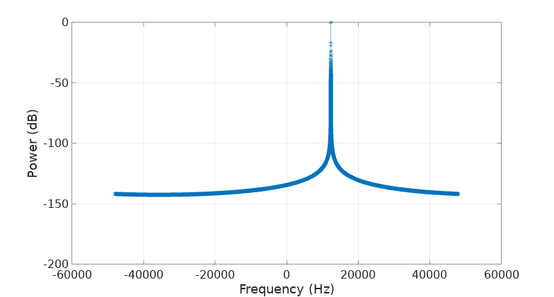

… the leakage is back!

Then the main topic of this article arises: how can the frequency of a phasor or carrier signal be estimated and how accurate can we get? Let’s do a zoom in to the first spectrum, the one produced with 1000 samples:

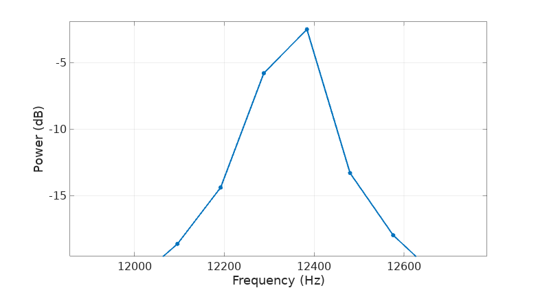
Because of our “incoherent” sampling we see how our phasor frequency doesn’t completely match one single frequency bin. If we have to say something, its frequency would be somewhere in between the bins at frequencies 12285 and 12384 Hz, probably closer to the later.

“Understanding DSP” by Richard Lyons offers a wonderful spectral peak location “trick”:

where \(X\) is the DFT of our signal, \(m_k\) is the bin for the maximum value in \(X\) and \(m_{k-1}\) and \(m_{k+1}\) are the previous and following bins respectively. This expression gives us an estimate for our phasor frequency of 12343.78 Hz which is indeed a very good estimate, within about 1 Hz from the exact result.

Lyon’s trick is however a bit short in explanations and references. Picked with interest, I’ll like to give it a go, following a path that has been traveled by many others before, to see where I get.

Derivation of a frequency estimation trick

I think I’m going to use the word “trick” instead of algorithm from now on. Anyway, given our phasor (including also an amplitude \(A\) and phase \(\theta\) for good measure):

and the DFT expression:

then

Thanks to the geometric sum formula, making \(r = e^{j 2 \pi (f/fs - k/N)}\) we get

where luckily \(e^{-j 2 \pi k}\) is 1 for all values of \(k\). Making \(a = e^{j 2 \pi f/fs}\) and \(b = e^{j 2 \pi/N}\) then

and therefore

It’s straightforward now to compute their ratio:

notice how the phase and amplitude cancelled out nicely. From here \(a\) can be derived:

and the frequency is computed as \(f = \dfrac{f_s}{2 \pi} atan2(imag(a), real(a))\),

In the absence of noise this is an exact expression, probably not far from Lyon’s one where he uses some more tricks to approximate the output from the atan2. However I’m not going to compromise here with accuracy because I believe the computation of this estimate is not expensive, just a few complex multiplications and an atan2 that can be evaluated with the help of lookup tables.

Additionally, having a general expression gives us the freedom to plug in different frequency bins and combine them to produce better estimates in the presence of noise. For instance, what I’m doing next is find the peak \(k\) in the spectrum and then do the average of the \(a\) values for \(i\) at [-2, -1, 1, 2], a couple of bins before and after the peak. Noise is added in steps to the input signal and the estimated frequency and its error are computed at each SNR level. The result looks like this:

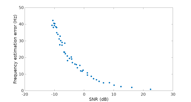
About 10 Hz of error at 0 dB SNR using a DFT of 256 points, or 0.08% of relative error, not bad. Below -10 dB the highest peak in the spectrum is not so likely to be the one from our phasor, completely messing up the estimation, but if you happen to roughly know the frequency you are looking for, then you can still expect this method to give you a decent estimate. Let’s then repeat the test doing some cheating, knowing that our phasor is at bin number 32:

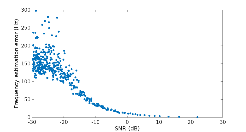
We can go down to a ridiculously low -20 dB SNR and still expect an error of about 150 Hz or 1.2% in relative terms (well, actually with fs = 96000 and a DFT of 256 points, each bin represents 375 Hz, if we know the bin of our phasor then we start with an uncentainty of +/- 187.5 Hz, so an error of +/- 150 Hz is nothing to write home about).

Let this thought be the closing of this topic for now.