Signal Derivative Considered Harmful?

Something you might have noticed if you follow the technology news is that whenever there is a problem with some complex artifact it turns out to be, in almost all instances, a software problem. At the time of this writing there is a particularly troubled North-American airplane and space manufacturer, see here, here and also here, that could give good testimony to this statement.

This happens more and more, but why? Is it because we, software engineers, still don’t know how to do our job right? Well, yes, but it also happens that software now is everywhere. Taking the discipline of radio communications as an example, the level of performance that a modern communication device requires can only be achieved with the execution of some complex computations. Those computations are what we call software and, as we try to keep squeezing the performance out of every corner, their complexity is going to keep increasing together with the number of lines of code and chances for mistakes.

Unfortunately software bugs are nothing new and they are not going away any time soon. There are many lessons we can learn from the mistakes of those who came before us. There are multiple references worth exploring, if not for our instruction, at least for the curiosity that the misfortune of others stimulate, similar to the impulse of turning our heads at a car wreck on the side of the road. One bad wreck was the popularly known as “the most expensive hyphen in history,” that resulted on the Mariner I LOM (loss of mission) on the fateful morning of July 22, 1962. The best account is probably in Pauls E. Ceruzzi’s 1989 book Beyond the Limits:

Timing for the two radar systems was separated by a difference of forty-three milliseconds. To compensate, the computer was instructed to add forty-three milliseconds to the data from the Rate System during the launch. This action, which set both systems to the same sampling time base, required smoothed, or averaged, track data, obtained by an earlier computation, not the raw velocity data relayed directly from the track radar. The symbol for this smoothed data was \(\bar{\dot{R}}_n\) or “R dot bar n,” where R stands for the radius, the dot for the first derivative (i.e., the velocity), the bar for smoothed data, and n for the increment.

The bar was left out of the hand-written guidance equations. Then during launch the on-board Rate System hardware failed. That in itself should not have jeopardized the mission, as the Track System radar was working and could have handled the ascent. But because of the missing bar in the guidance equations, the computer was processing the track data incorrectly. The result was erroneous information that the velocity was fluctuating in an erratic and unpredictable manner, for which the computer tried to compensate by sending correction signals back to the rocket. In fact the rocket was ascending smoothly and needed no such correction.

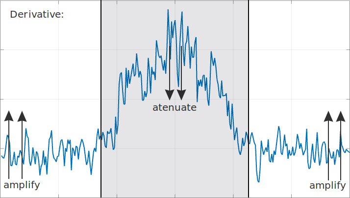
Why the missing bar (hyphen), or in other words, lack of smoothing over some data, was so critical? This is going to become the main subject of this article as you might have guessed from the title. My thesis here is that the smoothing of the data coming out from the derivative of the radius signal was a critical operation because the derivative is a dangerous operation. The derivative becomes dangerous when we engineers don’t take into account one of its side-effects and it is that it amplifies the noise. So to be honest to the truth, the real danger, as usual, lays down in our ignorance.

Let’s see what’s the truth behind this noise amplification statement. Once again we are not treading over unknown territory but instead we are standing over the shoulders of giants. I’m taking the Differentiators section from Richard G. Lyons’s Understanding Digital Signal Processing as reference and recommended lecture.

With all this preamble, let’s now roll up our sleeves and jump once again into the frequency domain with our trusty inverse discrete Fourier transform expression:

that says that a signal \(s\), whose samples are \(s(0)...s(N)\), can be expressed as a complex weighted summation of phasors, being the weights the complex values \(S(0)...S(N)\), also known as its “DFT coefficients.”

Since the derivative of a phasor is given by

Then the expression for the derivative of our signal becomes straightforward:

or in other words, what we are saying is that the DFT coefficients of the derivative of our signal are:

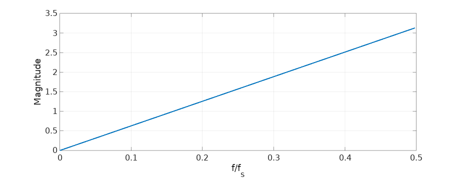
We have just calculated the transfer function of the derivative operation:

This expression sheds a lot of light into what the derivative does in the frequency domain. It tells us first that the frequency bins of our derivative are going to be translated in phase 90 degrees and there is also going to be a change in magnitude proportional to \(k\), so the coefficients at higher frequencies are going to be amplified more. We see this in the magnitude plot:

(and here in dB scale:)

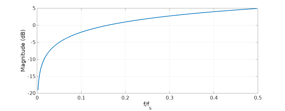
Considering the derivative as a filter, it’s an unusual one: it cancels completely the DC component and amplifies higher frequencies. This amplification is the troublesome part in the practical world where engineers dwell. In this world we are going to work with band-limited signals, signals that are sampled at some frequency that we choose high enough to capture completely our signal and with some margin to spare. We are also going to have noise, noise that is going to be ubiquitous. It’s going to look something like this in the frequency domain:

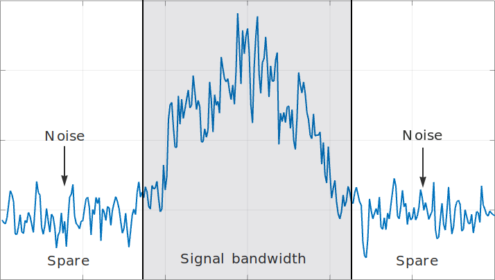
The important idea here is that the derivative of this signal is going to amplify up to 5 dB all that noise that shows up at the higher frequencies, outside of our signal’s bandwidth and it’s going to be amplified to a higher extent than our signal. Moreover, the lower frequency components of our signal are going to be attenuated, being its DC component completely removed.

We can intuitively see that the signal-to-noise ratio of our resulting derivative is going to suffer and we can end up with something that might look very different from what we expected. So much so the bigger the noise power in our spare bandwidth and the higher the concentration of power of our signal at the lower frequencies.

We can see that we need to be really careful here, but we haven’t reached the end of the story yet.

Practical implementation of the derivative

So far we have been talking about the derivative operation in its theoretical form. When it comes to its practical implementation we are going to be computing approximations to the derivative and we need to understand their properties and limitations.

Probably the first idea that come to our minds when we are tasked with computing the derivative of a signal in the digital domain is to put together something like this:

We compute the derivative (its approximation) as the difference of the current with the previous sample. This is called the first-difference differentiator and exploring its frequency response with Octave is a one-liner:

freqz([1 -1]);                      % First-difference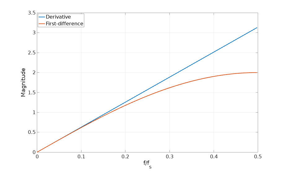

The approximation holds for the lowest frequencies but it’s not able to sustain the gain for higher frequencies:

We can compare this differentiator with another well-known expression:

This is called the central-difference differentiator and its frequency response can also be computed easily:

freqz([1 0 -1]/2);                  % Central-difference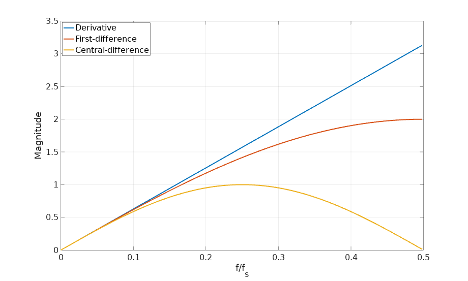

In this case we see how the frequency response for higher frequencies drops significantly. It might sound surprising, but this is actually a desirable characteristic. Remember that for bandwidth limited signals, the advice was to remove the out-of-band noise as much as possible. This differentiator offers both filtering and differentiation at the same time in a very simple expression. As long as our signal is sampled at 8 times or more its bandwidth (so we stay at \(f/f_s \lt 0.125\) in the chart), the central-difference will give us an accurate estimate without amplifying the noise at higher frequencies.

This low-pass filtering effect of the central-difference formula is expected since its expression is just the average of two consecutive first differences and we know that low-pass filtering, smoothing and averaging are all synonyms:

The theory from Savitzky-Golay filters give us even more options. If we are willing to increase the complexity, we can go to grades 5, 7 or 9:

freqz([2 1 0 -1 -2]/10);            % Savitzky-Golay, window size 5
freqz([3 2 1 0 -1 -2 -3]/28);       %         "         "         7
freqz([4 3 2 1 0 -1 -2 -3 -4]/60);  %         "         "         9

Let’s see what is their frequency response:

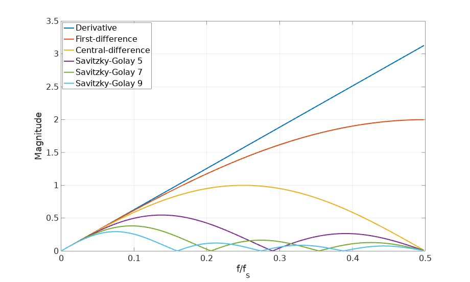
Notice how these higher order Savitzky-Golay filters are just focused on the smoothing of the results, filtering out the higher frequency components with still relatively simple expressions.

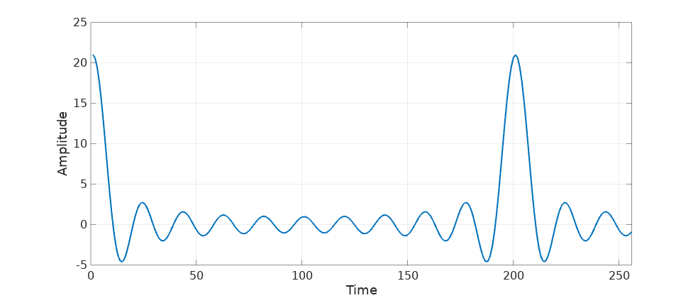
Is this the best we can do? Do we always need to trade accuracy and frequency response? No, as long as we are ready to bring more computing power to the table there is one more approach: design an ad-hoc differentiating filter that takes your exact signal sampling rate and bandwidth in full consideration. To illustrate this, let’s follow a practical example. Given this signal:

K = (0:255);
fs = 96000;
f1 = 4800;
N = 21;
df = f1/((N-1)/2);
SS = zeros(1, numel(K));
for ii=(0:N-1)
  SS = SS + exp(j*2*pi*K*(-f1+df*ii)/fs);
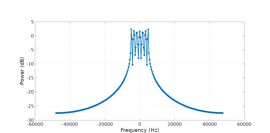
end

which is a composition of 21 phasors that cover 1/10 of the sampling frequency:

Computing the central-difference produces the following result:

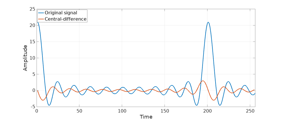
So far so good. Let’s add some white noise and repeat the computation:

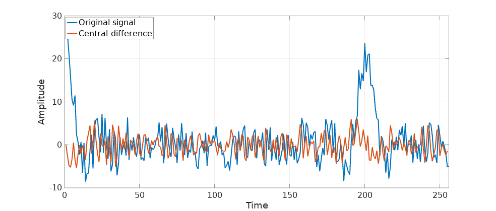
the derivative is barely recognizable:

That’s a lot of noise, probably even enough to crash a rocket. Let’s now design our ideal derivative filter for this particular signal. It should follow the ideal derivative frequency response (a straight line with slope \(2\pi\)) up to the signal bandwidth (which is 1/10 of our sampling rate) and drop to flat zero from then on.

It took me a while to tinker around with Octave’s remez function, probably other DSP tools can produce better results. This is as far as I got:

B = remez(60, [0 0.13 0.14 1], pi*[0 0.13 0.0 0], [1 1]);
B = B.*hamming(numel(B));

The additional application of a Hamming window is a nice improvement to reduce the filter’s ringing, as Mr. Lyons explains in the aforementioned reference.

The frequency response shows like this:

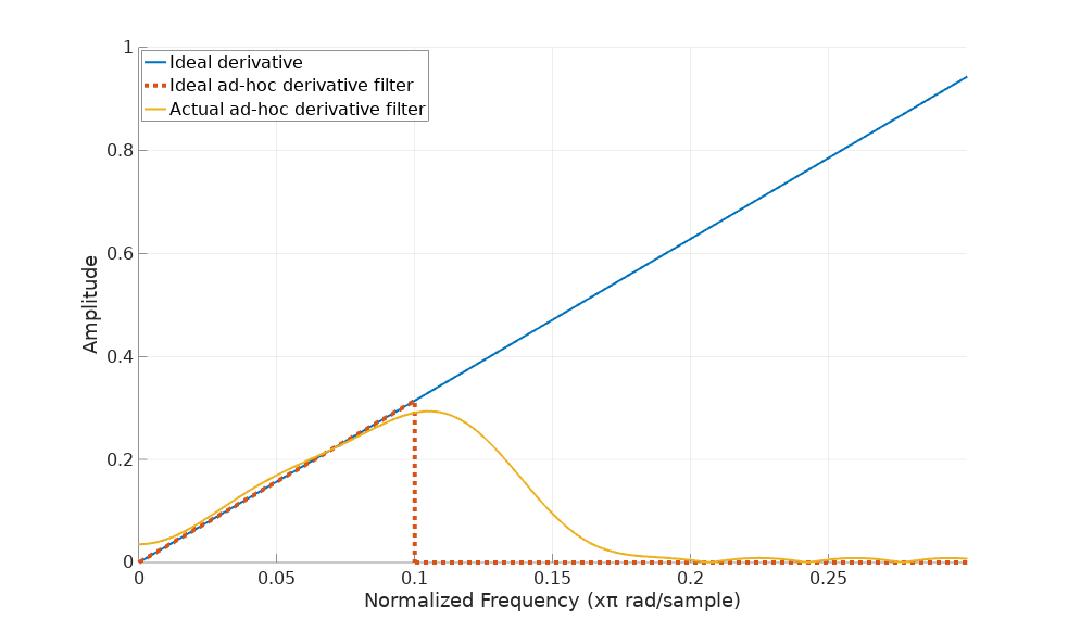
Quite close. We could make it even closer adding more taps but I think 60 are already quite a lot. Let’s see how if behaves with our input signal:

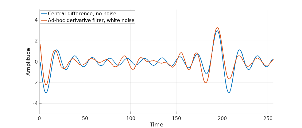
Not bad, the rocket has a better chance now. Notice that the output has been aligned in the plot to take into account the group delay that this filter produces.

With all these tools, it’s up to the particular scenario we face to choose the right one, making compromises where they can be safely made. Let a full understanding of our signal bandwidth and the impact of the noise be our guide to make the right choice in each circumstance. And let’s keep those rockets steady, even when the bars are left out of the requirements!