RF Direction Finding, Adcock/Watson-Watt Technique

I was involved some time ago on a project that used the Watson-Watt technique to estimate the direction of arrival of some radio signals. When I started I had zero knowledge on any of this direction finding (DF) business and getting the hang of it was not without difficulty. I can’t thank enough Ismael Pellejero and his excellent article, that really paved my way to the understanding of this technique. As a small token of gratitude to those who share their knowledge and experience, this is my try to extend on Mr. Pellejero explanations, given them an approach more focused on a software defined radio (SDR) practical implementation.

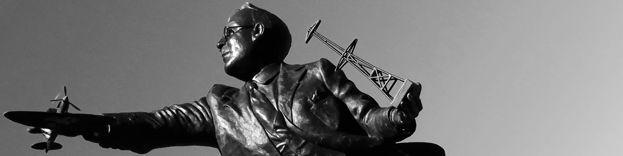
We are standing here upon the gigantic shoulders of Frank Adcock and Sir Robert Watson-Watt, WWII decisive heroes and complete no-ones outside radio or engineering circles (well, at least Sir Robert has a beautiful statue at his hometown). Why we are living in a society that picks their heroes among athletic games and show business celebrities, relegating the rest to oblivion will be the matter for another rambling. Today let’s remember that Sir Robert is non other than the father of radar and his biography explains how he experimented with the Adcock antenna array in the early 1920s, patented not long ago by Frank Adcock. The stroke of genius of Sir Robert was to make use of an oscilloscope to display graphically the angle of arrival of the radio signals. I can only imagine that using an oscilloscope in the 1920s would be equivalent to making use of a quantum computer or a similarly esoteric device in our more modern days.

But let’s dive into the details of this technique, which I believe is quite elegant. The configuration I’m going to consider for the Adcock antenna array is the one composed of five elements:

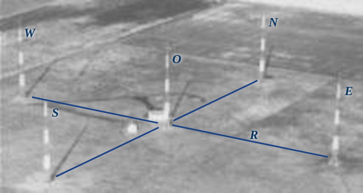
Those five elements are labeled accordingly as North (N), South (S), East (E), West (W) and arranged around the central “Omnidirectional” (O) element at an equal distance R. The photo depicts a large installation, probably meant for the LF/MF band and using, my guess, identical vertically polarized monopoles as antenna elements. Those elements must be wired in a particular way to conjure the DF magic. The North and South elements are combined in the following way to produce its difference at the output of the transformer:

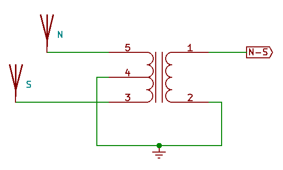
East and West elements are combined in the same way, whereas omni is left as it is. There are therefore three antenna outputs coming from this array: North minus South (NS), East minus West (EW) and Omni (O). Consequently, we are going to need for our radio frontend a receiver with three phase-coherent channels, all tuned to the same frequency. This is one of the advantages of this techniques: with only three channels, as we will see, we can produce a fairly accurate estimation of the angle of arrival of a signal covering 360°, as opposed to other more advanced techniques (I’m looking at you, beam-forming) that require more complicated hardware and antenna setups. Mind that in engineering complicated is often a synonym of expensive.

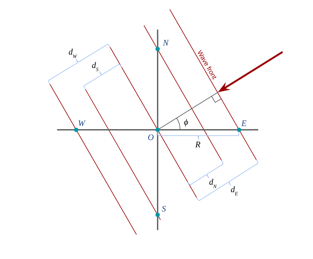
With this arrangement, let’s go with the classic diagram depicting a floor plan of our antenna array and a signal arriving from some particular angle, \(\phi\):

We take the O element as reference and we say that this element receives a signal \(r_O\):

It shouldn’t be a surprise that we consider our signal as a band-limited component \(m(t)\) that is carried at a frequency \(f_c\). We are ignoring noise at this point. We are also going to take advantage of the “far-field assumption,” that the signal has originated far away from our receiving antennas. We can then simply say that the wave front is flat and perpendicular to the direction of propagation (the perpendicular lines to the red arrow in the diagram).

It’s not difficult to see from the diagram that before reaching O, the signal has arrived earlier to E and N and will arrive later to S and W elements. How much earlier or later? That depends on the difference in the traveled distance and the signal’s propagation speed, which should be c in a vacuum, although we might not be in a vacuum, so let’s call it \(\nu\).

And it’s still not difficult to see that \(d_E\) (the additional distance the signal has to travel from the time it reaches E to the time it reaches O) is:

which is of the same magnitude as \(d_W\), and not surprisingly

also of the same magnitude of \(d_S\).

We can say then that our signal reaches element E at time

earlier that it does O, therefore the signal that E sees should be given by:

It’s time now to take another card from under our sleeve, this time is the “narrow-band assumption.” We claim that our m(t) signal is changing slowly, at least compared to the speed of change of our carrier frequency \(f_c\). To see how this is fair, let’s give some numbers, let’s say that we make R equal to one quarter of our wavelength \(\lambda\), and let’s say we are considering WiFi signals at 2.4 GHz, then our R is about 3.125 cm, which means a worst case time difference of about 0.1 nanoseconds to our radio signal. Considering that our WiFi signal has a bandwidth of 40 MHz, the highest frequency it’s going to carry is 20 MHz, which has a period of 50 ns. The compromise here is to say that a sinusoid with period 50 ns is not going to change much from time t to time t+0.1 ns. In fact we can say that the maximum change we are going to see with this delay in this example is about 1% (\(sin(2 \pi 0.1/50) \approx 0.0125\)).

Then we can simplify and say that:

Notice that we can’t ignore away the delay on the carrier component. In the example, a carrier of 2.4 GHz has a period of 0.4 ns, so a delay of 0.2 ns makes a significant difference. We can say that with an R equal or smaller that \(\frac{\lambda}{2}\), the difference in the signal that we are going to see is mostly coming from the phase difference of our carrier and very little from the changes in our base band signal m(t), whatever it might be.

We can extend this to the other elements:

So,

and since \(e^{j x} - e^{-j x} = cos(x) + jsin(x) - (cos(x) - jsin(x)) = 2jsin(x)\), then

with the consideration that \(\nu/f_c\) is the wavelength of our carrier frequency \(\lambda_c\):

and on the same fashion

This expresion can be simplified further. If we make \(R\) significantly smaller than \(\lambda_c\) we can make \(2 \pi \frac{R}{\lambda_c}\) small, so much so that we can claim that \(sin(x) \approx x\) for small values of \(x\), and

Those expressions are saying that \(r_{EW}\) and \(r_{NS}\) are either 90° ahead or behind of \(r_O\) (by the works of the imaginary unit \(j\) and the sign of the cosine and sine) and their magnitude is in proportion to that of \(r_O\) by a factor of the, respectively, cosine and sine of the signal’s angle of arrival \(\phi\).

If we divide the two expression we can recover the angle of arrival easily,

Or so it seems. The trouble here is that if we care to know what’s the quadrant our \(\phi\) is in, we need to know what’s the “sign” of both \(r_{NS}\) and \(r_{EW}\) and this is a tricky question because those are radio signals that we handle in our SDR implementation as a series of complex IQ samples, so it doesn’t make sense to ask about their sign by itself. We could, however, distinguish when both \(r_{NS}\) and \(r_{EW}\) are in phase or in opposition:

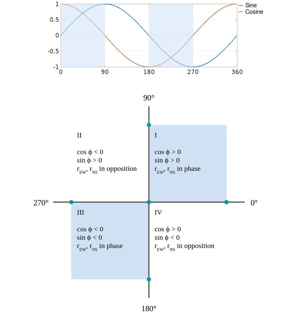
That will give us the ability to say if our signal is coming from either quadrants I, III or II, IV, but no more than that…

Or is it? Well, that’s true if we limit ourselves to only work with \(r_{EW}\) and \(r_{NS}\), but remember that we still have one more input signal, \(r_O\). This is the key to help us resolve exactly what quadrant we are in. Let’s see how.

It’s going to be useful to consider a phasor from our input signal \(r\). Let’s say it’s its the phasor corresponding to its strongest frequency component. If we represent together the phasors of all the signals coming to our antenna elements we would see something like this:

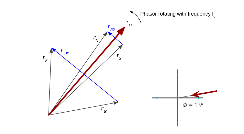
Following with our example where our signal is coming at an angle \(\phi\) that is in the first quadrant, and considering that our phasors are rotating counter-clockwise, we get that, respective to \(r_O\), \(r_N\) is ahead by a bit and \(r_S\) is behind by the same bit. The difference \(r_{NS}\) is logically at 90° with \(r_O\) and its magnitude goes with \(2 sin\phi\). Similarly, \(r_E\) is ahead of \(r_O\), this time by a significant amount and \(r_W\) is behind by the same amount, making \(r_{EW}\) again at 90° with \(r_O\) and with a magnitude that this time goes with \(2 cos\phi\). We see that both \(r_{NS}\) and \(r_{EW}\) are in phase, which is the expected in the first quadrant.

So far so good, let’s see what we get now for a \(\phi\) in the second quadrant:

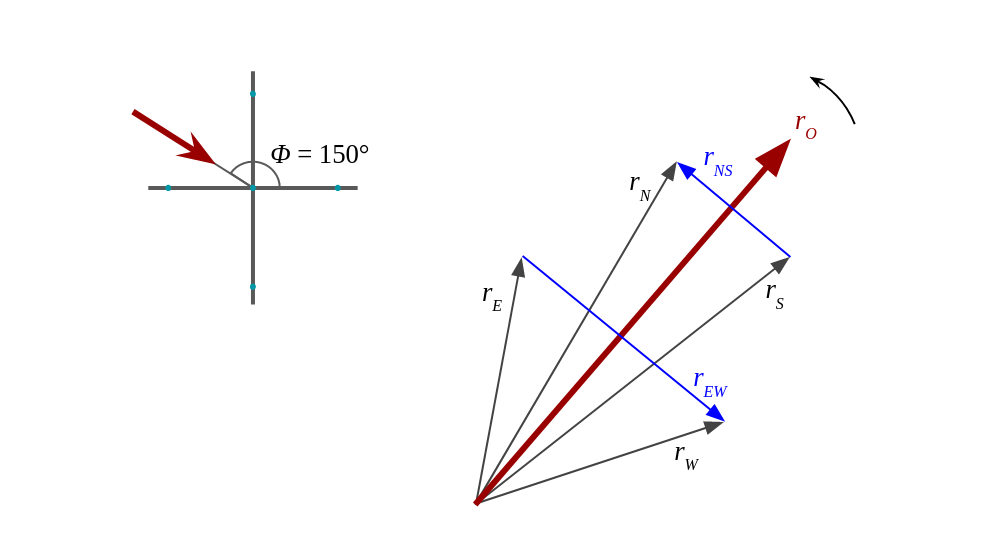
This time we see that \(r_E\) is early and \(r_W\) is late so the phase difference of \(r_{EW}\) with respect to \(r_O\) is minus 90°. And this is how we can determine which quadrant we are in: we compare the phase of our \(r_{NS}\) and \(r_{EW}\) with \(r_O\). This phase should be either plus or minus 90°. The sign will determine the quadrant we are in. In mathematical pseudo-code:

Where atan2 is the handy “2-argument arctan” than is present is so many programing environments and math computer tools.

And this should be the gist of this 100-year-old DF technique. I will conclude here for now with the idea of continuing with some more practical notes on a future article.