Analysis of the M&M Clock Recovery Algorithm

In my attempt to improve the AIS decoding software I run across a GNU Radio-based implementation that can be found at FunWithElectronics. This implementation uses the classical Mueller and Müller (M&M) timing recovery method. While trying to understand how it works I was misguided by several sources, wasted a lot of time and was about to give up. Finally I think I’m getting somewhere and I’m glad I did so I can move on with the rest of my life.

The main reference on this method is of course the original M&M paper ¹. It’s still possible to find it online looking up its title Timing Recovery in Digital Synchronous Data Receivers. The authors propose a new family of timing recovery methods where the ADC is going to work at the signal symbol rate. This is already an impressive accomplishment and probably what called my attention in the first place. Consider the case of the GNU AIS software were the sampling rate is five times the signal symbol rate. Seems like a timing method that works at just the symbol rate should require in the order of five times less computing resources. That’s interesting.

Let’s take a look at how this is possible. For a transmission system with overall impulse response \(h(t)\), transmitted symbols \(a_k\) and noise \(n(t)\), the signal that we receive is modeled as:

or in simplified notation

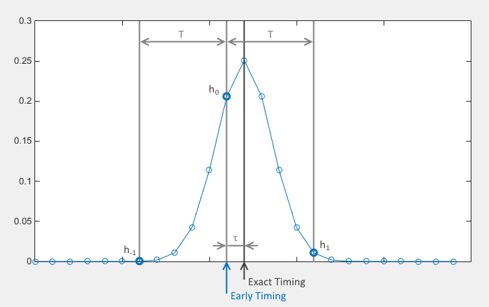
Trying to stay focused on the context of AIS, the impulse response of a GMSK signal is a Gaussian function whose “roll-off” is governed by its BT product. For the case of AIS, ITU recommends a BT product equal to 0.4. That looks more or less like the blue plot in the figure:

(See this Matlab article for more details on how to produce the plot.)

M&M show how consecutive samples measured regularly at the symbol rate can convey timing information. In the above figure the peak of the Gaussian should be the sample we read if our timing is right on the spot, but if we are late (by \(\tau\), the sampling phase) we are going to read \(h_0\) instead. In the previous sampling period (T seconds ago, being T the symbol period) we did read \(h_{-1}\) and in the next sampling period we will read \(h_1\). In this case we can see how the difference \(h_1 - h_{-1}\) is going to be negative, indicative that we need to decrement our timing phase to synchronize with the transmitted signal.

It’s already clear, but for completeness let’s examine an example of early timing:

Here the sign is reversed, \(h_1 - h_{-1}\) is now positive, indicative that our timing phase needs to increase.

The authors then present the Type A timing function as:

We can see in the following chart that in fact this function is very much correlated to the sampling phase:

So given \(h_1\) and \(h_{-1}\) we calculate our \(f\) and we increase or decrease out sampling phase accordingly. This is great but we still have a long way ahead before the method becomes practical. The issue is that on the receiving side we never see the individual impulse responses for each transmitted symbol. What we get is \(x(t)\), the superposition of the delayed responses for each transmitted symbol.

The genius of the M&M method is to derive a simple approximation whose expected value is the same as our \(f(\tau)\):

being

That’s it, on average, \(z_k\) tends to be equal to our timing function and we can use this value to adjust our sampling phase. This expression is dependent of the symbols transmitted \(a_k\), that’s why this method is cataloged as “decision-directed feedback.” Certainly we don’t know what symbols were transmitted, we can only make a decision on what symbols we think were transmitted, based on the \(x_k\) values we receive. For a bipolar encoding we can decide that \(a_k = -1\) (bit 0) if \(x_k \lt 0\) and \(a_k = 1\) (bit 1) if \(x_k \ge 0\) (notice that we are counting that \(x(t)\) is not affected by any DC bias).

I have expended most of the time in trying to find out from a quantitative point of view whether this approximation works or not. In some particular cases it seems that it doesn’t, that the method is a pointless idea. For instance:

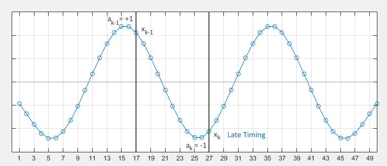
The sequence “01010” that we sample late. Clearly the peaks and valleys are symmetric and at \(k=27\) (T is 10 in this example) the value of \(x_{17} = -x_{27}\). Then

therefore, no problem whatsoever with the sampling phase is detected, we get under the impression that our timing is perfect, which is not the case. Is the problem that this method cannot be applied to GMSK signals? Is it something else? Well, no. The method only claims that it is the expected value of \(z_k\) that should get equal to our timing function. Let’s see how it in fact works. Let’s take the 32 possible combinations of 5 binary symbols and the expected \(x(t)\) that we should receive in each case. The following figure is the superposition of all of them (I’m not yet considering the addition of noise):

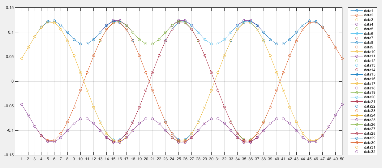
Where data1 corresponds to the sequence 00000, data2 = 00001,… up to data32 = 11111.

With a simple script we can evaluate the different values of \(z_k\) at different samples for each sequence and calculate their mean values. I’m going to focus on the third transmitted symbol (right in the middle). We can see how the results in the next figure follow a familiar shape:

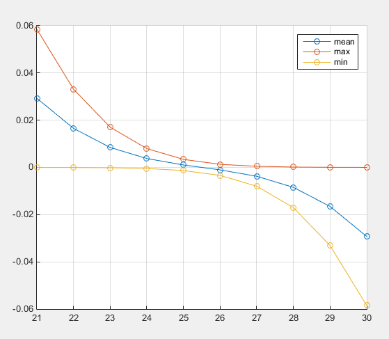
The mean, in blue, matches very well the shape of our timing function \(f(\tau)\). We can also see how in some cases the \(z(k)\) we obtain is zero, like in the previous example. So it can be criticized that with some unfortunate long data combination the method won’t work (M&M only claim that this method is valid for equally distributed symbols).

My conclusion is that the method works in principle with GMSK signals. I don’t want to make this article any longer and I stop here leaving for the next one an evaluation of the method applied to some real AIS signals. I will use the M&M implementation that comes with GNU radio, which will also give me a chance for its analysis.

References

K. Mueller and M. Muller, “Timing Recovery in Digital Synchronous Data Receivers,” in IEEE Transactions on Communications, vol. 24, no. 5, pp. 516-531, May 1976, doi: 10.1109/TCOM.1976.1093326. ↩
Leave a Comment