Analysis of the GNU Radio M&M Clock Recovery Implementation

In this second part of the analysis of the Mueller and Müller (M&M) timing recovery method I’m going to focus on the GNU radio implementation and evaluate its performance when applied to AIS signals.

The first consideration is that even though one of the key achievements of the M&M algorithm is its ability to work at the same sampling rate as the symbol period (9600 Hz for AIS), in the GNU radio implementation we see how the signal is sampled instead at 50 kHz (~5.2 samples per symbol). The reason is that on modern SDR systems the software layer doesn’t have the ability to control directly the sampling rate on the ADC, usually residing in a different piece of hardware. M&M was designed in 1976 to be implemented in hardware and connected to the ADC clock reference. We can scratch our heads immediately considering whether or not M&M is a good option for an SDR implementation. An algorithm that is designed to work at the symbol rate but actually works with signals sampled at a higher rate seems to be in disadvantage when compared to algorithms that are natively designed to work at higher sampling rates.

With this consideration let’s directly dive into the GNU radio implementation. The code can be found at gr-digital/lib/clock_recovery_mm_ff_impl.cc and it’s fairly concise:

int
clock_recovery_mm_ff_impl::general_work(int noutput_items,
                                        gr_vector_int &ninput_items,
                                        gr_vector_const_void_star &input_items,
                                        gr_vector_void_star &output_items)
{
  const float *in = (const float *)input_items[0];
  float *out = (float *)output_items[0];

  int ii = 0; // input index
  int oo = 0; // output index
  int ni = ninput_items[0] - d_interp->ntaps(); // don't use more input than this
  float mm_val;

  while(oo < noutput_items && ii < ni ) {
    // produce output sample
    out[oo] = d_interp->interpolate(&in[ii], d_mu);
    mm_val = slice(d_last_sample) * out[oo] -
             slice(out[oo]) * d_last_sample;
    d_last_sample = out[oo];

    d_omega = d_omega + d_gain_omega * mm_val;
    d_omega = d_omega_mid +
              gr::branchless_clip(d_omega-d_omega_mid, d_omega_lim);
    d_mu = d_mu + d_omega + d_gain_mu * mm_val;

    ii += (int)floor(d_mu);
    d_mu = d_mu - floor(d_mu);
    oo++;
  }

  consume_each(ii);
  return oo;
}

In the FunWithElectronics reference mentioned in the previous article the member variables we see in the code are initialized as follows:

• d_omega = 50000 / 9600 = 5.20833
• d_gain_omega = 0.25 * 0.175 * 0.175 = 0.00765625
• d_mu = 0.5
• d_gain_mu = 0.175
• d_omega_relative_limit = 0.005
• d_omega_mid = d_omega
• d_omega_lim = d_omega_mid * d_omega_relative_limit

Here d_omega is the symbol period in samples (T in the M&M paper). We see how the FunWithElectronics implementation is expecting that the AIS signal is sampled at 50 kHz, being 9600 the AIS symbol rate.

d_mu is our symbol phase. It works exactly as \(\tau\) in the M&M paper, being its range [0,1]. I’ll explain this further in a bit.

d_gain_omega and d_gain_mu are the gains of the proportional-integral feedback loop we will talk about later. d_omega_relative_limit sets a limit to the value that d_omega can vary. In this implementation is set to ±0.5% of d_omega.

Once the meaning of these constants is clear we can start to understand what the code is doing. We see how inside the while loop the first thing is to get the interpolated value of the input signal, given the current sample index and the symbol phase d_mu:

    out[oo] = d_interp->interpolate(&in[ii], d_mu);

This is the way modern SDR systems overcome the lack of direct control over the ADC clock: to work at increased sample rates and do an interpolation to estimate the value of the signal at an arbitrary symbol phase.

d_interp is an interpolating FIR filter (mmse_fir_interpolator_ff) with 8 taps. It’s important to understand how it works because it can lead to confusion:

Let’s say that we call the interpolate method with address \(in\) and let’s say that there we have the samples \([in_0, in_1, in_2, in_3, in_4, in_5, in_6, in_7, ...]\). The interpolating filter is going to use samples \(in_0\) to \(in_7\) and produce an interpolated value between the central samples \(in_3\) and \(in_4\) according to the value of d_mu: with d_mu=0 the interpolated value should return exactly \(in_3\), with d_mu=1 it should return exactly \(in_4\), and with d_mu=0.5 it should return the interpolated value midway between them. In practice the effect is that this filter introduces a delay of 3 samples although this is not going to affect the timing algorithm in anyway as we will see.

The next line is the gist of the synchronization and having analyzed the theory behind M&M on the previous article it should look pretty familiar at this point:

    mm_val = slice(d_last_sample) * out[oo] -
             slice(out[oo]) * d_last_sample;

Just a quick side note because we haven’t seen yet the slice method. It’s the symbol estimator, the module that decides if the symbol is a one or a zero:

static inline float
slice(float x)
{
  return x < 0 ? -1.0F : 1.0F;
}

If the sample is negative, it is a zero (-1). Otherwise is a one (+1). It can’t be simpler than this.

Therefore slice(d_last_sample) is the \(a_{k-1}\) from the M&M paper, out[oo] is the \(x_k\), slice(out([oo])) is \(a_k\) and d_last_sample is \(x_{k-1}\), so

which is the value whose expected value converges to the M&M timing function and that we can use to adjust our symbol phase d_mu and symbol period d_omega.

This adjustment is exactly what is happening in the next lines.

    d_omega = d_omega + d_gain_omega * mm_val;
    d_omega = d_omega_mid +
              gr::branchless_clip(d_omega-d_omega_mid, d_omega_lim);
    d_mu = d_mu + d_omega + d_gain_mu * mm_val;

    ii += (int)floor(d_mu);
    d_mu = d_mu - floor(d_mu);

The symbol phase is adjusted proportionally to the calculated mm_val. As it was explained in the previous article, when the timing is late the M&M timing function returns a negative value, indicative that we should decrement our phase and, likewise, when the timing is early the value is positive so we should increment our phase. The d_gain_mu is the proportional constant in our control loop and the rational behind the selection of this particular value of 0.175 is never explained, although it seems to be working well as we will see later.

The symbol period is adjusted with the d_gain_omega in a similar way. I will call this the integral constant since the symbol period can be interpreted as the integral of the symbol phase. Its value is two orders of magnitude lower than the proportional constant and this makes sense since the symbol period shouldn’t require any significant adjustment (according to ITU the transceiver characteristics for AIS set a tolerance of ±50ppm). Additionally there is a cap to how much the symbol period can vary. The branchless_clip call limits the variation to ±0.5% of the default symbol period as defined in the d_omega_relative_limit constant.

Let’s see next how this method performs with some real AIS signals. I’m benchmarking this method comparing the timing with what I call “exact” timing determined by examining the signal’s eye diagram, similarly to what was done on the first article of this series Clock Recovery in GNU AIS.

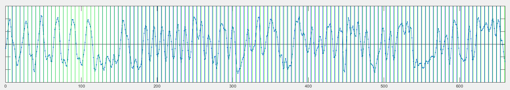
First an example of an AIS transmission where the M&M algorithm works very well:

The timing instants calculated with the M&M code are superimposed as vertical blue lines together with the “exact” timing in green. As can be seen they are consistently very close together.

The difference between the timing instants is plotted next:

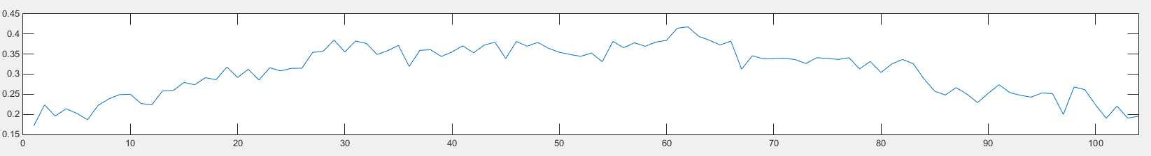
We can see how the method performs well and after a number of samples the phase error is reduced. The units of the vertical axis are sample periods. Since the sampling rate is ~5.2 times the symbol rate, the maximum error of 0.4 represents an error of ~7.7% of the symbol period (0.4*100/5.2). Mind that an error of 50% of the symbol period is already a total disaster since we will be sampling our symbols at the very same sample where the zero-crossings are supposed to occur.

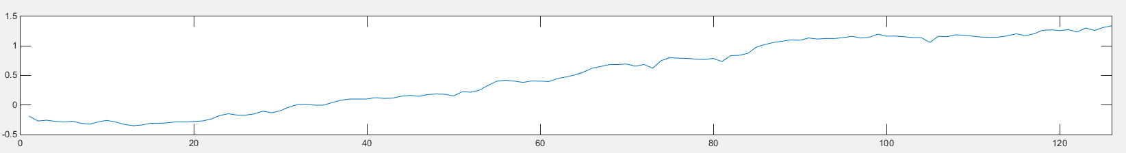
Let’s see with a longer AIS message how the M&M timing behaves. On the next example we see how once the timing error accumulates in one direction exceeding some threshold it bounces to the opposite direction:

The highest error that I have observed with the GNU AIS “Helsinki” dataset (the GNU AIS gnuais-stereo-2rx.raw channel A) is about 1-1.5 samples or about 19-29% of the symbol period.

Let’s take a look now at an example of a bad bit estimation consequence of poor timing:

And the timing error:

The timing starts well but slowly grows surpassing the 1 sample mark without a sign yet of bouncing down. Let’s take a closer look to sample 445 where the timing makes a decisive double mistake:

The red circles highlight the sample values read by the M&M method and in green the samples than the exact timing would read. We can see how they are at different sides of the 0 voltage and therefore will be interpreted as different symbols by the slice method, being the M&M interpretation incorrect. At this point the timing is off by just one sample (or about 20% of the symbol period) but this is already high enough to make a double mistake. We have then an example of how AIS signals sampled at ~5.2 samples per symbol require a timing accuracy better than 20% the symbol period for a consistent symbol estimation.

In this particular example the timing function is not converging fast enough to the correct timing phase and the feedback loop is not able to notice the accumulated error to bring it down. But in general the M&M timing function does an great job. Over the “Helsinki” dataset, the latest GNU AIS code (analyzed two articles ago) successfully decodes 115 AIS messages. A modified version of the code using the M&M timing function reaches 178 messages, a significant improvement.

The conclusion is that the M&M algorithm works and it works better with AIS signals than the original GNU AIS timing function. I tried with different values of the feedback loop gains (d_gain_omega, d_gain_mu) but I didn’t achieve significant improvements. I’ll need more data to be able to fine tune those constants. Even though the authors of FunWithElectronics don’t give out any information on how those values have been chosen, they seem to work well.

I’ll conclude here this article. It has been a long journey for me to reach some of the secrets inside the M&M timing function and I hope this information can be useful to whoever has an interest in this rather esoteric matters.

On the next article I will explore a different synchronization technique I have tried during the course of this analysis and that is able to produce results closer to the “exact” timing already mentioned.