An Improved Clock Recovery Algorithm for AIS

After analyzing the clock recovery algorithms of GNU AIS as well as the GNU radio implementation based on the M&M method, I’m going to give my take on an alternative algorithm that seems to be working well, at least for AIS signals.

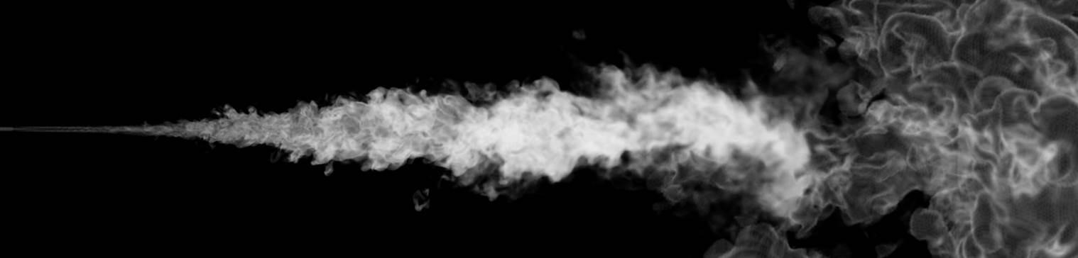
In the first article in this series I was working with an AIS signal transmission that challenged the GNU AIS implementation:

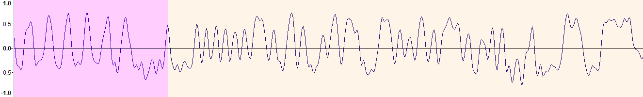
(the purple background color highlights the training sequence plus start flag). That article also presented the signal’s differential phase eye diagram, which can be produced by knowing in advance the correct number of samples per symbol (SPS). In this case we know that SPS should be near 5 since the sampling rate is 48 kHz and the symbol rate is 9600 bauds:

The eye in this diagram looks clean and with a wide opening, sufficient to decode the signal correctly, provided that the timing phase could be determined. Moreover, we can see how there is no significant timing drift comparing the training sequence plus start flag (purple color) from the rest (orange). This is expected since the whole signal transmission that we are looking at here lasts only 13.5 ms.

Let’s do now the exercise of finding out the locations of the zero-crossings on the eye diagram. We are aware that the eye diagram is a representation of the original signal’s phase difference “wrapped” in time by the SPS value. This wrap is nothing but a modulus operation. To give a numerical example, let’s say the the zero-crossings are happening at instants \(T = [0.81, 9.89, 20.21, ...]\), on our eye diagram with \(SPS = 5\) they would show at \(mod(T, SPS) = [0.81, 4.89, 0.21, ...]\).

The wrapped zero-crossings look like this:

On the left we see the equivalent of the eye diagram but only showing the signal where it crosses zero. Notice how the values wrap around from left to right, which indicates that a polar diagram (on the right) is a more adequate representation.

This polar representation give us the hint on how to look for the signal’s timing phase: interpret those wrapped zero-crossings as angles and estimate its average. In this particular example the average is \(0.26\), which means that \(0.26 + SPS/2 = 2.76\) is the center of our “eye” in our eye diagram, which seems about right.

The code to run this computation is like this:

/**
 * \brief Estimates the signal's timing phase as the location of the signal's zero-crossings.
 * \param a_signal The pointer to the array of signal samples.
 * \param a_offset An offset into the array.
 * \param a_samples Number of samples available in the array.
 * \param a_SPS Number of samples per symbol
 * \param a_zero Zero signal value.
 * \return The averaged zero-crossings location as a fraction of a_SPS.
 */
float estimate_timing_phase(const int16_t* a_signal, const unsigned int a_offset, const unsigned int a_samples, const float a_SPS, const int16_t a_zero)
{
    float sum_cos = 0.0f;
    float sum_sin = 0.0f;
    //unsigned int n = 0;

    const int16_t* p_signal = a_signal + a_offset;
    int16_t last_value = *(p_signal++);
    bool last_value_gt_zero = (last_value >= a_zero);

    for(unsigned int i=1; i<a_samples; i++) {
        int16_t value = *(p_signal++);
        bool value_gt_zero = (value >= a_zero);
        // Check for a zero crossing
        if (value_gt_zero != last_value_gt_zero) {
            // Simplest lineal interpolation to find more exactly where the zero crossing happens
            float x = ((float)last_value) / ((float)(last_value - value));
            float crossing = ((float)(i - 1)) + x;

            // Find its SPS modulus
            crossing = fmod(crossing, a_SPS);
            // Normalize to [0,2*PI]
            float crossing_pseudo_angle = crossing * 2.0f * (float)M_PI / a_SPS;
            // Accumulate
            sum_cos += cos(crossing_pseudo_angle);
            sum_sin += sin(crossing_pseudo_angle);
            //n++;
        }
        last_value = value;
        last_value_gt_zero = value_gt_zero;
    }

    // Find the average angle. Actually we don't need to divide by n, atan2 is already normalizing the values
    //float offset = atan2(sum_sin / (float)n, sum_cos / (float)n);
    float offset = atan2(sum_sin, sum_cos);
    // Translate back to sample units
    offset *= a_SPS / (2.0f * (float)M_PI);

    return offset;
}

I hope it’s simple enough. The signal values are checked detecting for zero-crossings. Once one is found, a simple linear interpolation produces a decimal estimate of the location of the crossing (the x variable in the code will be closer to 0 when abs(last_value) is small compared to abs(value) and closer to 1 the other way around). The crossing location is wrapped by applying the modulus with a_SPS, converted into an angle in the range \([0,2\pi]\) and its sine and cosine accumulated to later produce the average sine and cosine (see this wikipedia article on how to calculate averages of “circular” quantities).

That’s all there is to it. As I already mentioned, this code produces the estimate of \(0.26\) when applied over the total 649 samples of this AIS signal transmission we are using as an example. When applied only over the initial 125 samples, which corresponds to just the training sequence, the estimate is \(0.16\), being then the center of the “eye” at \(0.16 + SPS/2 = 2.66\), which is still a good value. From the previous figure we can see how the opening in the eye is approximately in the range \([1.5,4.3]\). Any estimate in between this range is not going to produce any timing error whatsoever.

Let’s now pit this algorithm (which I’m going to refer to as Rolling Barnacle, or RB) with the previous ones, using the same “Helsinki” benchmark:

This timing algorithm is able to decode correctly 208 messages from the benchmark dataset, a 80% improvement over the original GNU AIS implementation and 17% over the M&M.

The decoding procedure has been modified slightly. It can be summarized in the following steps:

1. Detection of the training sequence and start flag.
2. Estimation of the timing phase so far using the RB algorithm.
3. Detection of the end flag, but no decoding yet. Estimation of the DC component (the a_zero argument on the estimate_timing_phase function).
4. Estimation again of the timing phase, this round using the whole signal segment (from the beginning of the training sequence to the end flag).
5. Extract symbols and decode.

Note that this algorithm is not adapting the timing phase as the signal progresses. Even though it assumes that there is no timing drift, it’s still able to produce good results since it’s using the whole signal segment to produce an excellent (optimal?) estimate of the timing phase.

As far as its computational performance, it can be said that the RB algorithm described here might be heavier that the other methods we have analyzed so far. It makes use of trigonometric functions (although those can be implemented with lookup tables) and requires more memory (the whole signal needs to be placed in a buffer since we are making three rounds over it). These can be a consideration for embedded silicon but for modern CPUs it shouldn’t be an issue.