
Power analysis for direct sampling and direct conversion SDR designs
With the advancement of analog-to-digital converters (ADCs) capable of higher sampling frequencies, the “direct sampling” approach in software-defined radio (SDR) is gaining significant traction. While I’m not the expert in the nuances of this design in comparison with the more traditional “direct conversion” method, this note aims to provide a fundamental analysis of how both signal and noise powers are impacted in each approach. By exploring these effects from first principles, we are going to touch into some important signal processing concepts.
We start selecting a single tone at frequency \(f_c\) as our input signal:
\[r(t) = A cos(2 \pi f_c t + \phi_0)\]By its definition, its power can be calculated as:
\[P_r = \mathbb{E}[|r(t)|^2]\]Where \(\mathbb{E}[\cdot]\) denotes the expected value operator, which, in our context, corresponds to the time-average over a long period:
\[P_r = \lim_{T \to \infty} \frac{1}{2T} \int_{-T}^{T} |r(t)|^2 dt = \lim_{T \to \infty} \frac{1}{2T} \int_{-T}^{T} A^2 cos^2(2 \pi f_c t + \phi_0) dt\]Using
\[\int cos^2(a x + b) dx = \frac{2 (a x + b) + sin(2(a x +b))}{4a}\]we get
\[P_r = \lim_{T \to \infty} \frac{A^2}{2T} \left[ \frac{4 \pi f_c t + 2 \phi_0 + sin(4 \pi f_c t + 2 \phi_0)}{8 \pi f_c} \right]_{-T}^{T} =\] \[= \lim_{T \to \infty} \frac{A^2}{2T} \frac{4 \pi f_c T + 4 \pi f_c T + sin(4 \pi f_c T + 2 \phi_0) - sin(- 4 \pi f_c T + 2 \phi_0)}{8 \pi f_c} =\] \[= \lim_{T \to \infty} \frac{A^2}{2T} \frac{8 \pi f_c T + 2 cos(2 \phi_0)sin(4 \pi f_c T)}{8 \pi f_c} =\] \[= \lim_{T \to \infty} \frac{A^2}{2} + \frac{A^2cos(2 \phi_0)sin(4 \pi f_c T)}{8 \pi f_c T} = \frac{A^2}{2}\]The power of a \(cos\) wave (same for \(sin\), since the difference between the two is just some phase offset) with amplitude \(A\) is \(A^2 / 2\).
Direct conversion

The signal \(r\) is split in two, half of the power goes to each output of the splitter where they are mixed respectively with a \(cos\) and \(sin\) signals, with frequency the central frequency of our interest.
Signal analysis
On an idealized splitter, the output signals \(r_i\) and \(r_q\) should each have half the power of the original signal. We will find that these output signals should be:
\[r_i(t) = \frac{1}{\sqrt{2}} r(t)\] \[r_q(t) = \frac{1}{\sqrt{2}} r(t)\]We can easily calculate their power:
\[P_{r_i} = P_{r_q} = \lim_{T \to \infty} \frac{1}{2T} \int_{-T}^{T} \left\lvert \frac{r_i(t)}{\sqrt{2}} \right\rvert ^2 dt = \frac{P_r}{2}\]validating that it’s indeed half of the power of the original signal.
On the next step we are going to mix these outputs with \(sin\) and \(cos\) signals respectively. This is performed in the analog domain. To maintain an accurate balance of powers, we account for the amplitudes of the \(sin\) and \(cos\) signals, assuming that it’s the same, \(M\), for both and ignoring their initial phases, which we assume it’s also the same and equal to 0:
\[m_i(t) = M cos(2 \pi f_c t)\] \[m_q(t) = M sin(2 \pi f_c t)\]In this fashion, we can calculate their power:
\[P_{m_i} = P_{m_q} = \frac{M^2}{2}\]We take a note here that to have unit power, we need to make \(M = \sqrt{2}\).
After the frequency mixing (mixing = multiplication) our components become:
\[r_i(t) = \frac{M}{\sqrt{2}} r(t) A cos(2 \pi f_c t)\] \[r_q(t) = \frac{M}{\sqrt{2}} r(t) A sin(2 \pi f_c t)\]And since
\[cos(x+y)cos(x) = \frac{1}{2} \bigl( cos(2x+y) + cos(y) \bigr)\] \[cos(x+y)sin(x) = \frac{1}{2} \bigl( sin(2x+y) - sin(y) \bigr)\]We get:
\[r_i(t) = \frac{MA}{\sqrt{2}} cos(2 \pi f_c t + \phi_0) cos(2 \pi f_c t) = \frac{MA}{2 \sqrt{2}} \bigl( cos(2 \pi 2 f_c t + \phi_0) + cos(\phi_0) \bigr)\] \[r_q(t) = \frac{MA}{\sqrt{2}} cos(2 \pi f_c t + \phi_0) sin(2 \pi f_c t) = \frac{MA}{2 \sqrt{2}} \bigl( sin(2 \pi 2 f_c t + \phi_0) - sin(\phi_0) \bigr)\]An interesting exercise is to calculate the power of these two components. Applying the steps that we have already presented, we can find that:
\[P_{r_i} = \frac{M^2 A^2}{8}(\frac{1}{2} + cos^2(\phi_0))\] \[P_{r_q} = \frac{M^2 A^2}{8}(\frac{1}{2} + sin^2(\phi_0))\]so
\[P_{r_i} + P_{r_q} = \frac{M^2 A^2}{8}(1 + sin^2(\phi_0) + cos^2(\phi_0)) = \frac{M^2 A^2}{4}\]Having \(M=\sqrt{2}\) for unit power at the mixing signals makes the sum of these two powers equal to \(A^2 / 2\), the same power we started with, which is a good sanity check.
Back to our direct conversion, the next step is to low-pass filter our signal with the purpose of removing the components at the \(2f_c\) frequency. With the appropriate filter we should be able to remove completely the components at two times \(f_c\) leaving our signal of interest at baseband unaffected. We should find out that we are left with:
\[r^\prime_i(t) = \frac{MA}{2 \sqrt{2}} cos(\phi_0)\] \[r^\prime_q(t) = -\frac{MA}{2 \sqrt{2}} sin(\phi_0)\]After the ADC, the samples of these two signals are combined in the digital domain as the real and imaginary components of a complex-valued signal:
\[r^\prime(t) = r^\prime_i(t) + i r^\prime_q(t) = \frac{MA}{2 \sqrt{2}} \bigl( cos(\phi_0) - i sin(\phi_0) \bigr)\]where \(i\) is the imaginary unit. The power of this signal (now reduced to a DC component) is:
\[P_{r^\prime} = \mathbb{E}[|r^\prime(t)|^2] = \mathbb{E}[\Re \bigl( r^\prime(t) \bigr) ^2 + \Im \bigl( r^\prime(t) \bigr)^2)] = \Biggl( \frac{MA}{2 \sqrt{2}} \Biggr) ^2 \bigl( cos^2(\phi_0) + sin^2(\phi_0) \bigr)\] \[P_{r^\prime} = \frac{M^2 A^2}{8}\]With \(M=\sqrt{2}\) the power would be \(A^2 / 4\). This is half the power that we started with. Where did we lose the other half of the power? Into the \(2 f_c\) components that we filtered out. Is this a problem? No, we will see why when we conduct the same analysis for the noise power next.
Noise analysis
We start with a random normal variable with mean 0 and variance equal to its squared standard deviation \(\sigma_{n}\):
\[n(t) \sim \mathcal{N}(0,\sigma_{n}^{2})\]As it goes though the splitter and frequency mixer, we apply the same transformations:
\[n_i(t) = \frac{M}{\sqrt{2}} n(t) cos(2 \pi f_c t)\] \[n_q(t) = \frac{M}{\sqrt{2}} n(t) sin(2 \pi f_c t)\]One interesting point that we are going to use later is that, after multiplying by \(cos\) and \(sin\) respectively, \(n_i(t)\) and \(n_q(t)\) have become uncorrelated. See appendix A for the detailed derivation.
But let’s calculate the power of the \(cos\) component:
\[P_{n_i} = var[n_i] = \mathbb{E}[n_i^2] - (\mathbb{E}[n_i])^2 =\] \[= \mathbb{E}[ ( \frac{M}{\sqrt{2}} ) ^2 n^2(t) cos^2(2 \pi f_c t) ] - (\mathbb{E}[\frac{M}{\sqrt{2}}n(t) cos(2 \pi f_c t)])^2 =\] \[= \frac{M^2}{2} \mathbb{E}[ n^2(t) cos^2(2 \pi f_c t) ] - \frac{M^2}{2}(\mathbb{E}[n(t) cos(2 \pi f_c t)])^2\]The expected value of \(cos^2\) is \(\frac{1}{2}\), the expected value of \(cos\) is 0, and the expected value of \(n^2(t)\) is \(\sigma_{n}^{2}\), then
\[P_{n_i} = \frac{M^2}{2}\sigma_{n}^{2}\frac{1}{2} - 0 = \frac{M^2}{4}\sigma_{n}^{2}\]The \(sin\) component should have the same power:
\[P_{n_q} = \frac{M^2}{4}\sigma_{n}^{2}\]After low pass filtering, the noise power should be reduced accordingly to the fraction of frequencies that our filter allows to pass through, relative to our sampling rate. Let’s call this ratio \(\alpha\). Then
\[P_{n^\prime_i} = \frac{M^2}{4}\sigma_{n}^{2} \alpha\] \[P_{n^\prime_q} = \frac{M^2}{4}\sigma_{n}^{2} \alpha\]These filtered components, after they are sampled in the ADC, form our real and imaginary components in the digital domain:
\[n^\prime(t) = n^\prime_i + i n^\prime_q\]And since the filtered signals continue to be uncorrelated, its power is the sum of the powers of the real and imaginary components:
\[P_{n^\prime} = P_{n^\prime_i} + P_{n^\prime_q} = \frac{M^2}{2}\sigma_{n}^{2} \alpha\]The final noise power depends on the bandwidth of our low-pass filter. If we had \(M=\sqrt{2}\) for unit power at the mixer, and no filtering (\(\alpha=1\)), we would have \(P_{n^\prime} = \sigma_{n}^{2}\), which is the same noise power we started with. With a half-band filter (\(\alpha=0.5\)), the final noise power will be halved and since the signal power is also halved, we end up with an unmodified signal-to-noise ratio (SNR).
Direct sampling
The direct sampling design strikes us with its beautiful simplicity:
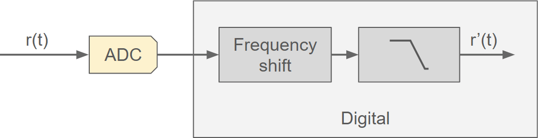
Signal analysis
We start with the same input signal:
\[r(t) = A cos(2 \pi f_c t + \phi_0)\]This signal is directly sampled (hence the name) and, already in the digital domain, it gets frequency shifted, producing components:
\[r_i(t) = r(t) M A cos(2 \pi f_c t) = \frac{MA}{2} \bigl( cos(2 \pi 2 f_c t + \phi_0) + cos(\phi_0) \bigr)\] \[r_q(t) = r(t) M A sin(2 \pi f_c t)= \frac{MA}{2} \bigl( sin(2 \pi 2 f_c t + \phi_0) - sin(\phi_0) \bigr)\]These signals have double the power that their equivalent in direct conversion. The reason is that in the digital domain we don’t need to split the signal in half-power components. In digital processing, multiple operations can be performed on the same signal without physically splitting its power, unlike analog systems.
Since the frequency shifting is also in the digital domain, we would usually make \(M=1\), but let’s leave it indicated for an easier comparison with the previous analysis on direct conversion.
The components at \(2 f_c\) frequency are again filtered out, this time in the digital domain. We are left with:
\[r^\prime_i(t) = \frac{MA}{2} cos(\phi_0)\] \[r^\prime_q(t) = -\frac{MA}{2} sin(\phi_0)\]which are reinterpreted as the real and imaginary components of a complex-valued signal:
\[r^\prime = r^\prime_i(t) + i r^\prime_q(t) = \frac{MA}{2} \bigl( cos(\phi_0) - i sin(\phi_0) \bigr)\]with power
\[P_{r^\prime} = \frac{M^2A^2}{4}\]This is twice the value we calculated for direct conversion. But let’s see what happens to the noise before comparing results for both designs.
Noise analysis
In a similar fashion, we get:
\[n(t) \sim \mathcal{N}(0,\sigma_{n}^{2})\]There is no splitter, just frequency shifting:
\[n_i(t) = n(t) M cos(2 \pi f_c t)\] \[n_q(t) = n(t) M sin(2 \pi f_c t)\]Their power should be the same and can be calculated as:
\[P_{n_i} = P_{n_q} = var[n_i] = \mathbb{E}[n_i^2] - (\mathbb{E}[n_i])^2 =\] \[= \mathbb{E}[ n^2(t) M^2 cos^2(2 \pi f_c t) ] - (\mathbb{E}[n(t) M cos(2 \pi f_c t)])^2 =\] \[= \frac{M^2}{2}\sigma_{n}^{2}\]After filtering
\[P_{n^\prime_i} = P_{n^\prime_q} = \frac{M}{2}\sigma_{n}^{2} \alpha\]so
\[P_{n^\prime} = n^\prime_i + i n^\prime_q = M^2\sigma_{n}^{2} \alpha\]which is also twice the value that we calculated for direct sampling.
Results summary
| Baseline | Direct conversion | Direct sampling | |
|---|---|---|---|
| Signal power | $$ \frac{A^2}{2} $$ | $$ \frac{M^2 A^2}{8} $$ | $$ \frac{M^2 A^2}{4} $$ |
| Noise power | $$ \sigma^2_n $$ | $$ \frac{M^2 \sigma^2_n \alpha}{2} $$ | $$ M^2 \sigma^2_n \alpha $$ |
| SNR | $$ \frac{A^2}{2 \sigma^2_n} $$ | $$ \frac{A^2}{4 \sigma^2_n \alpha} $$ | $$ \frac{A^2}{4 \sigma^2_n \alpha} $$ |
Since both signal and noise power are doubled with direct sampling, in comparison with direct conversion, there is no difference in the resulting SNR. In fact, with direct sampling the gain introduced by \(M\) is in the digital domain, so it’s always our design choice. The choice of a digital gain is based on the consideration of keeping the scaling of the signal such that it fits comfortably in the number of bits that our digital processing computing device provides.
With \(M=\sqrt{2}\) for a mixer that doesn’t alter the signal power, we find that direct conversion loses half of the original signal power. That half of the power we can say is lost at the low-pass filter that removes the components at two-times \(f_c\). The direct sampling design presented here also implements a low-pass filter that also removes half of the power, however in direct sampling the absence of an analog splitter has the effect of doubling the signal power. That’s why with direct sampling the signal power remains unchanged.
Appendix A
Multiplying white noise by \(sin\) and \(cos\) makes these two random variables uncorrelated. How do we know this? We can check their covariance. Uncorrelated random variables should have zero covariance.
From its definition:
\[cov(n_i, n_q) = \mathbb{E}[(n_i - \mathbb{E}[n_i])(n_q - \mathbb{E}[n_q])]\]where the expected value for both \(n_i\) and \(n_q\) should be zero, then:
\[cov(n_i, n_q) = \mathbb{E}[n_i n_q] = \mathbb{E}[\frac{1}{\sqrt{2}} n(t) cos(2 \pi f_c t) \frac{1}{\sqrt{2}} n(t) sin(2 \pi f_c t)]\] \[= \mathbb{E}[\frac{1}{2} n^2(t) cos(2 \pi f_c t) sin(2 \pi f_c t)] \tag{1}\label{eq:1}\]We invoke at this point the definition for variance of a random variable X:
\[var[X] = \mathbb{E}[X^2] - (\mathbb{E}[X])^2\]therefore
\[\mathbb{E}[X^2] = var[X] + (\mathbb{E}[X])^2\]applied to our \(n(t)\):
\[\mathbb{E}[n(t)^2] = \sigma_{n}^{2} + 0 = \sigma_{n}^{2}\]This allows us to go back to our expression \((1)\) and take the constant values out of the expectation:
\[cov(n_i, n_q) = \frac{1}{2} \sigma_{n}^{2} \mathbb{E}[cos(2 \pi f_c t) sin(2 \pi f_c t)]\]and since \(cos(x)sin(x) = \frac{1}{2}sin(2x)\):
\[cov(n_i, n_q) = \frac{1}{2} \sigma_{n}^{2} \mathbb{E}[\frac{1}{2} sin(2 \pi 2 f_c t)]\]The expected value of the \(sin\) function is zero, which makes the whole covariance zero, proving that \(n_i\) and \(n_q\) are indeed uncorrelated.
Leave a Comment