RF Direction Finding, Adcock/Watson-Watt Technique (II)

As a continuation of the previous article on this subject, I’m going to discuss this time some practical considerations based on my experience with this direction finding (DF) technique.

The analysis of this technique yielded a straightforward expression for $\varphi$, the estimated angle of arrival of our signal of interest:

where

and $r_{NS}$, $r_{EW}$ and $r_O$ are the three outputs coming out of our Adcock antenna into our 3-channel coherent radio receiver.

Effects of the approximations

Remember that to reach those expressions we made a number of assumptions:

The far field assumption

Our receiving antenna is far away from our transmitter of interest, so much that the wave front can be considered a plane instead of what really is, the surface of a sphere. Since engineers are trained to simplify cows into spheres, it should not be a big jump to further simplify a sphere into a plane. This can be considered a safe assumption in most practical applications.

The narrow band assumption

We claim that the highest frequency component of our base band signal is much lower that our carrier frequency. For most practical cases this will be true but to quantify the effect, let’s take a baseband signal of bandwidth $W$, its highest frequency component will then be $f_m=W/2$. With a carrier frequency $f_c$, it will have rotated 360° in a period equal to $\frac{1}{f_c}$. During that same time, the baseband signal should have then changed $e^{j2\pi \frac{1}{f_c}{f}_m}=e^{j\pi \frac{W}{f_c}}$.

We can plugin some numbers to get the feeling of it: in the 70 cm band with a signal of 25 kHz of bandwidth, the value we get from our little formula is $e^{j1.8e-4}$, which is a rotation of 0.01°. Very little in comparison.

The ratio antenna array radius (R) to signal wavelength is small

With small values of $2\pi \frac{R}{\lambda }$ we can simplify a $sin$ from our expressions and produce the very compact one at the top of this article, that involves just an arctan operation. This is probably the trickiest one. A reason why it might not be the case that this ratio is not so small is because we might want our DF setup to operate in a wide range of frequencies and being our antenna array a rigid installation, we might be pushing the limits at higher frequencies (lower $\lambda$).

Another reason might be, and I’m not an antenna expert, that antenna arrays with elements spaced so close in comparison to the signal’s wavelength, have strong electromagnetic interactions and each individual element pattern is not individual any more but affected greatly by the other elements. How this interaction plays, whether positively or negatively, I would like to understand better (but my bet is that it’s going to be negative).

Considering that this assumption doesn’t hold, our expressions get more verbose:

Let’s run some simulations with different values or $R/\lambda$ next to see what we get.

Using the example from Mr Pellejero’s technical article, at a frequency of 5 MHz we get a $\lambda$ of 60 m. Placing our antenna elements at R = 7.5 m, or $\lambda /8$, we get $2\pi \frac{R}{\lambda }=0.78$ and making $r_O=1$, our $r_{NS}$ and $r_{EW}$ look like this:

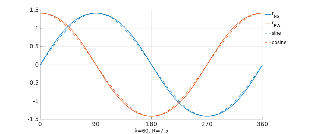
Quite close to the true sine and cosine curves, so in this case the arctan approximation should not be a problem.

Making R twice this value, or one quarter of our wavelength, starts to show a clear distortion:

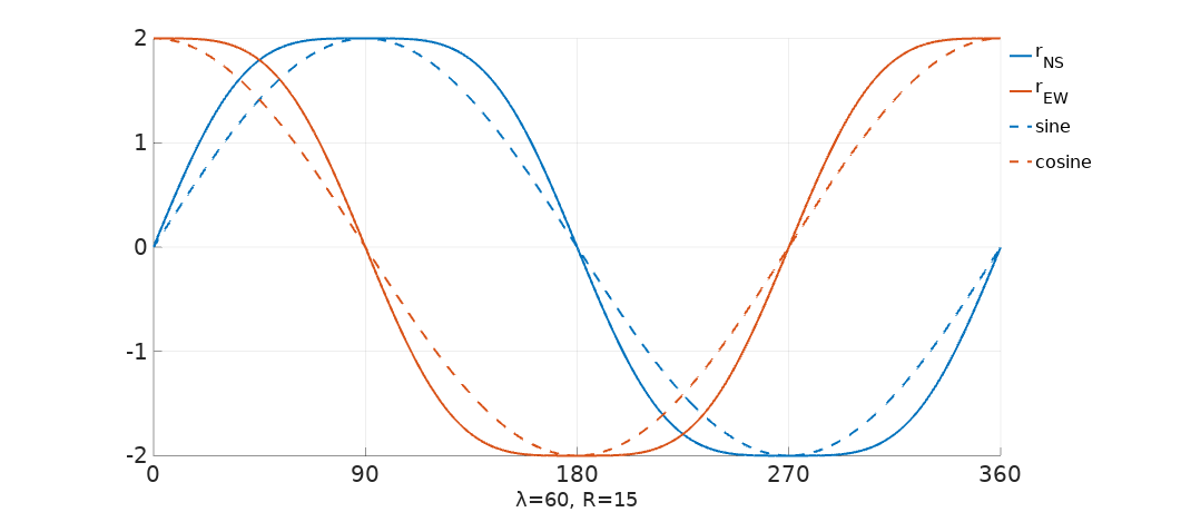
Our peaks have got flatten at $90n$ and at $90n+45$ degrees the error with the true sine and cosine is now evident. What I say in this case is that we don’t need to compromise. I can understand the justification for the simplification a century ago, but these days we carry in our pockets millions of times more computing power that what was used to land the man on the moon. At any rate, a software defined radio (SDR) implementation of the Watson-Watt DF method is not going to make a call to atan2. It should be much faster to use a lookup table and, once the decision to use a table is made, the content of the table doesn’t need to be produced from perfect sine and cosine values, it will use the actual distorted but more accurate values that we see here and the processing unit is not going to tell the difference.

So, what we do is to take our antenna setup to a calibration session, either to an anechoic RF chamber or some remote outdoor location, we take measurements around 360° and take note of the power ratios $r_{NS}/r_O$ and $r_{EW}/r_O$. With these values we build our lookup tables, then, we don’t need to worry about this effect since we are compensating exactly for it.

In fact we could say that this distortion can be compensated advantageously because when one $r$ becomes flatter (and therefore it loses ability to resolve), then the slope on the other $r$ is the most pronounced (and therefore with the highest ability to resolve). So, f.i. around 90°, $r_{NS}$ is going to return a value of around 2 for a wide margin of angles, but it doesn’t matter because $r_{EW}$ is changing very rapidly in this neighborhood so it will tell us precisely what angle our signal is coming from.

Or does it? No, not really.

Accuracy and some experimental results

Sorry for giving false hope but it isn’t going to work out. All said is correct but the problem here is that the points with the maximum slope are also the points where our $r$ is the smallest. Being small means that the readings are most likely dominated by noise, not the signal. So, on the one hand we have, let’s continue with 90° as an example, a $r_{NS}$ strong but dumb and on the other we get $r_{EW}$ with random values coming from the noise. It isn’t going to look good.

Before we jump into conclusions, let’s see first some results coming from the calibration of a particular Adcok antenna at some particular band:

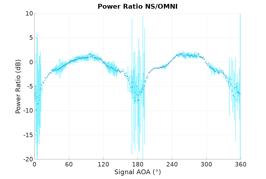
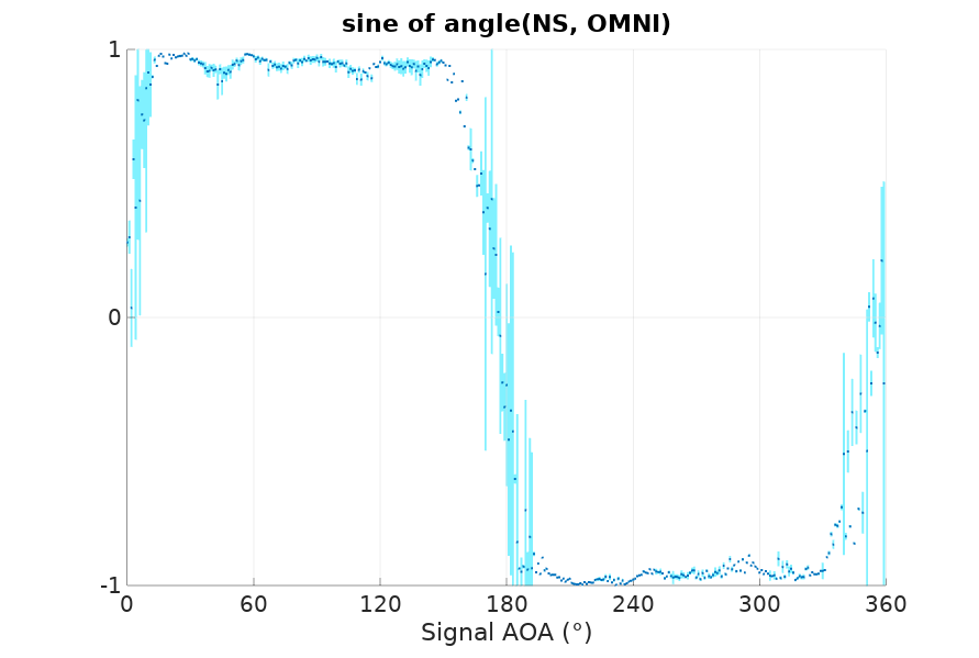
The first chart is $\frac{\Vert r_{NS}\Vert }{\Vert r_O\Vert }$, the magnitude ratio of $r_{NS}$ and $r_O$, and the second is the sine of the angle between $r_{NS}$ and $r_O$. The darker dots are at the average and the lighter color bars represent the standard deviation. Remember that $r_{NS}$ and $r_O$ should be at either plus or minus 90°, so the sine should be either 1 or -1, and that is pretty much what we get, being the regions around 0 and 180 degrees quite noisy for the reasons explained before. If you multiply the magnitude of the first chart with the sign from the second chart, you would obtain something that follows a sine, with several distortions. Some expected like the flattening around 270°, and some others that might be explained as undesired electromagnetic interactions between antenna elements, the mast or other nearby components.

We get analogous results for $r_{EW}$:

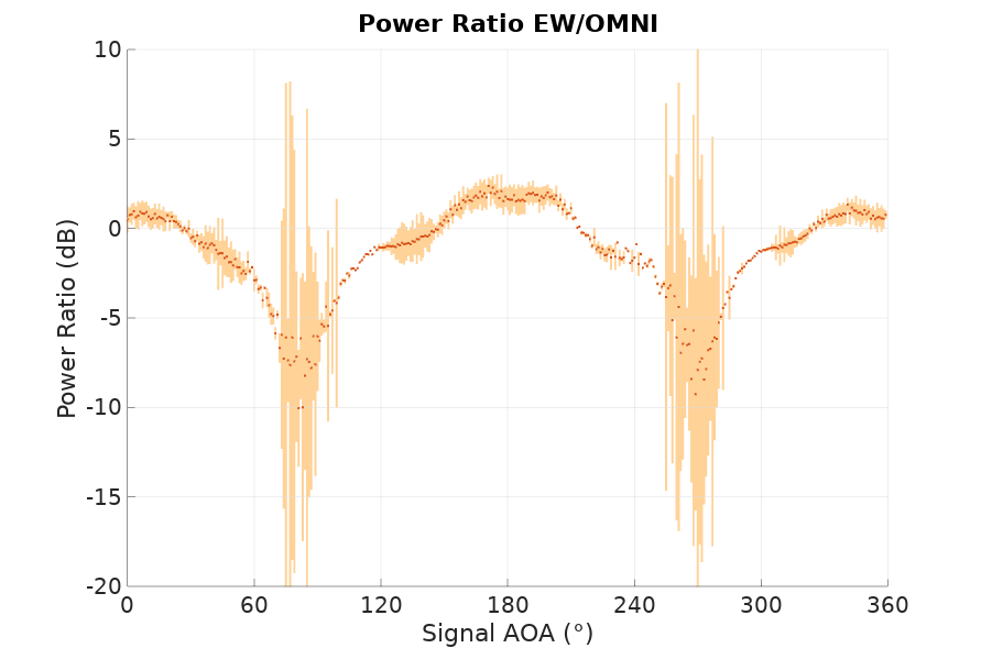
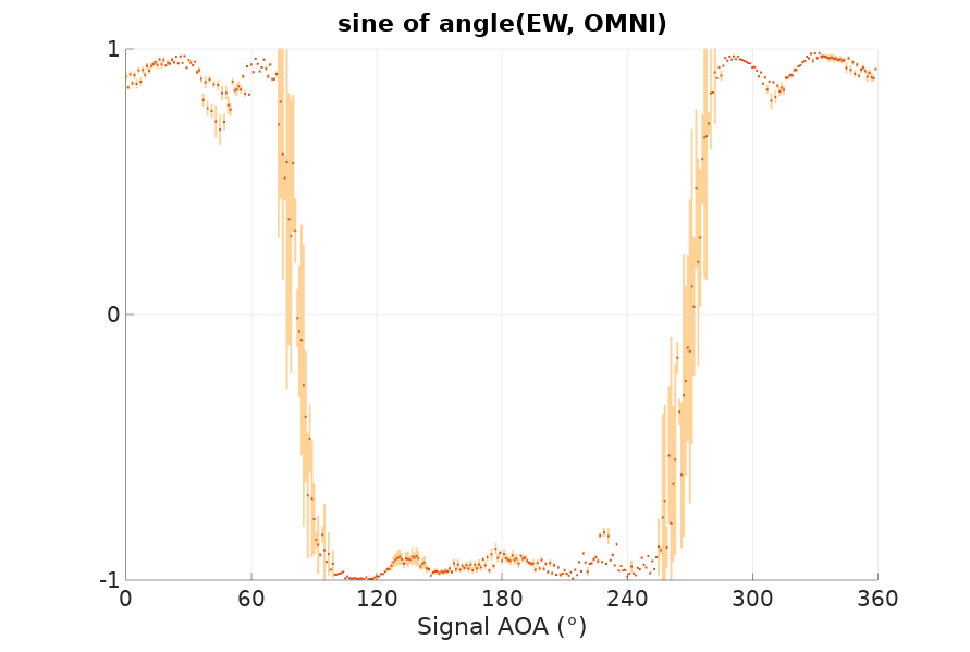
In this case the multiplication of the magnitude ratios from the first chart with the sign from the second chart would give us something that follows a cosine, with some distortions as expected.

Let me reiterate that the purpose of calibration is to understand those distortions from the textbook sine and cosine ideal shapes. Once we take them into account in our computations, they should not be detrimental to the accuracy of our results. The real problem of this technique is the nulls that the antenna array produces at 0, 90, 180 and 270 degrees. I believe this is the weakest point of this DF technique and its limiting factor to produce a high level of consistent accuracy.

Is there anything we can do to improve things? Yes, there are a couple of things we can do. If accuracy is the concern, we can spend more money and come up with two sets of Adcock antennas rotated 45° respective of each other, so when our transmitter is at $90n$ degrees to one of them (low accuracy expected), it will be at $90n+45$ degrees to the other (not so low accuracy). One could say that, for the cost of two sets of Adcock antennas and two sets of 3 channel coherent radio receivers, one could put together a 6-antenna element beam-forming solution with superior accuracy. And that one would be right but there is something very cool you can do with two Adcock antennas that you can’t do with a 6 channel beam former: You can cross the streams!

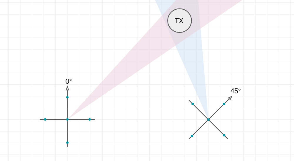
And by doing so you’ll find that you have transcended the realm of direction finding and you are now dwelling with the Gods in the realm of geo-location.

There is one more option that occurs to me and this one is easier with your wallet: you filter the noisy DF estimations with a Kalman filter, which I believe is ideal for this kind of application, particularly if you are dealing with moving transmitters and you happen to get some idea of their dynamics, such as speed and trajectories they might follow or some constrains on them.

I still haven’t talked about some implementation details that I believe are interesting. I’ll leave that for the next and last article in this series.